Application of stable isotope probing to identify temperature responsive bacterial taxa at the level of 3-hydroxy fatty acid synthesis: Time T3 and T7
in progress
collaboration
Authors
Affiliation
Olivier Rué
Migale bioinformatics facility
Christelle Hennequet-Antier
Migale bioinformatics facility
Published
November 22, 2023
Modified
February 19, 2025
Note
This document is a report of the analyses performed. You will find all the code used to analyze these data. The version of the tools (maybe in code chunks) and their references are indicated, for questions of reproducibility.
Aim of the project
The aim of the project is to provide a better understanding of how soil bacteria respond to temperature variations at the membrane level. Bacterial lipids can be used in paleoclimatology to reconstruct temperature of past climates in marine and terrestrial archives. This involves the use of proxies and calculations that are based on the relative amounts of these lipids. In soil, only one organic proxy is available, mainly due to the difficulty to work on soil, which is much more heterogeneous in structure than aquatic environments. A drawback of this sungle proxy is the error which is associated with it as well as the lack of confirmation of the result by a different approach. A new proxy based on 3-hydroxy fatty acids has been proposed in 2016. To better understand and validate this proxy, as well as to investigate new more precise proxies, we aim at understanding what soil bacterial species contribute to the proposed proxy by investigating their response te temperature at the taxonomic and lipid levels. We have used a DNA- and lipid-SIP approach during a time-course experiment and are now at the stage of analyzing what species have used the 13C labelled substrate in a temperature dependent manner. The profile of the enriched taxa in the 13C fraction will be compared in the different samples (different temperature, different incubation time) and will be compared with the 13C-enriched lipid profiles in the same samples.
Deliverables agreed at the preliminary meeting (Table 1).
Table 1: Deliverables
Definition
1
HTML report
Data management
Important
All data is managed by the migale facility for the duration of the project. Once the project is over, the Migale facility does not keep your data. We will provide you with the raw data and associated metadata that will be deposited on public repositories before the results are used. We can guide you in the submission process. We will then decide which files to keep, knowing that this report will also be provided to you and that the analyses can be replayed if needed.
Biostatistics
The phyloseq package[1] is a tool to import, store, analyze, and graphically display complex metabarcoding data, especially when there is associated sample data, phylogenetic tree, and/or taxonomic assignment of the OTUs or ASVs. Various customs functions written to enhance the base functions of phyloseq are available in the phyloseq-extended package[2].
[[1]]
[1] "1] Min. number of reads = 10643"

[[2]]
[1] "2] Max. number of reads = 48037"

[[3]]
[1] "3] Total number of reads = 4010689"

[[4]]
[1] "4] Average number of reads = 29708.8074074074"

[[5]]
[1] "5] Median number of reads = 31149"

[[6]]
[1] "7] Sparsity = 0.218730882381593"

[[7]]
[1] "6] Any OTU sum to 1 or less? NO"

[[8]]
[1] "8] Number of singletons = 0"

[[9]]
[1] "9] Percent of OTUs that are singletons \n        (i.e. exactly one read detected across all samples)0"

[[10]]
[1] "10] Number of sample variables are: 10"

[[11]]
 [1] "Time"                   "Temperature"            "SampleID"
 [4] "Replicate"              "FractionOnCsClGradient" "Glucose"
 [7] "Temperature_NotOrd"     "Time_Gluc"              "Group"
[10] "SampleLabel"
Show the code
saveRDS(object = physeq, file="physeq.rds")
Show the code
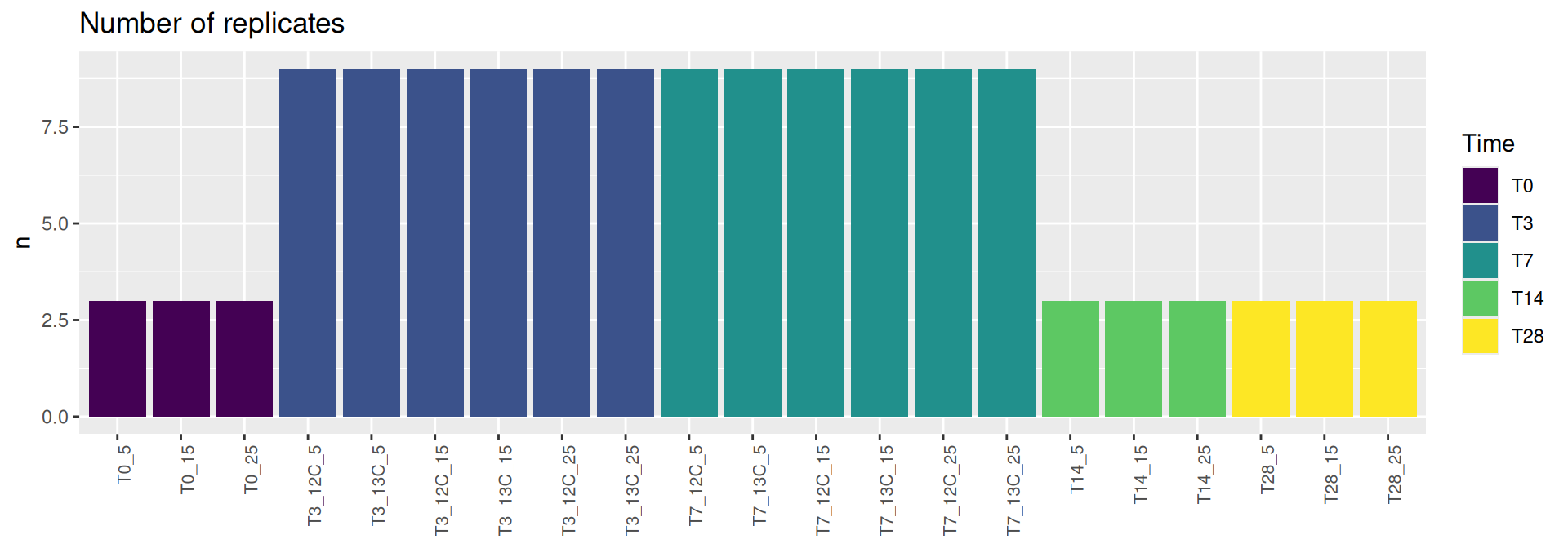
# count number of samples per conditionsample_data(physeq) %>%as_tibble() %>% dplyr::count(Time)
# A tibble: 5 × 2
  Time      n
  <ord> <int>
1 T0        9
2 T3       54
3 T7       54
4 T14       9
5 T28       9
Show the code
sample_data(physeq) %>%as_tibble() %>% dplyr::add_count(Time, Temperature, Glucose) %>% dplyr::select(Time, Temperature, , Glucose, Group, n) %>%distinct() %>%ggplot(., aes(x = Group, y = n, fill = Time)) +geom_bar(stat ="identity") +labs(title="Number of replicates", y ="n") +theme(axis.title.x =element_blank(),axis.text.x =element_text(angle =90, size =8, hjust =1))
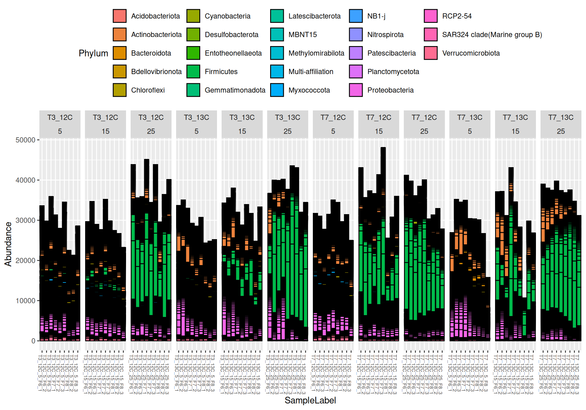
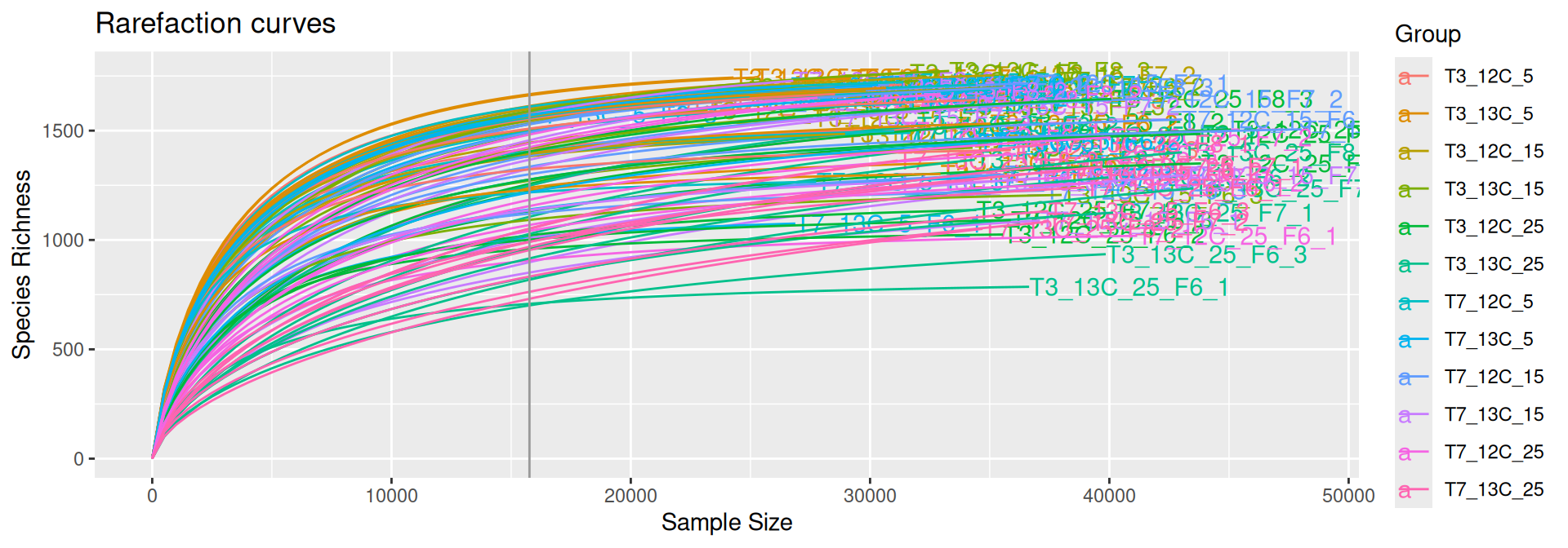
The common practice for comparing microbiome samples of different library sizes is to reduce the size of the larger samples using rarefaction until they contain the same number of reads as the smallest sample. The rarefaction curves show the species richness (i.e. number of species) against the library size and the vertical grey line indicates the smallest sample’s size. Each curve indicates when the sampling depth is sufficient to achieve an acceptable number of species discoveries and when increasing the depth leads to the discovery of rarer species. Rarefied data are used to estimate and compare alpha and beta diversity across samples.
Problematic taxa
                 taxa  Kingdom      Phylum  Class   Order  Family rank
Cluster_23 Cluster_23 Bacteria Chloroflexi KD4-96 Unknown Unknown    9
Results
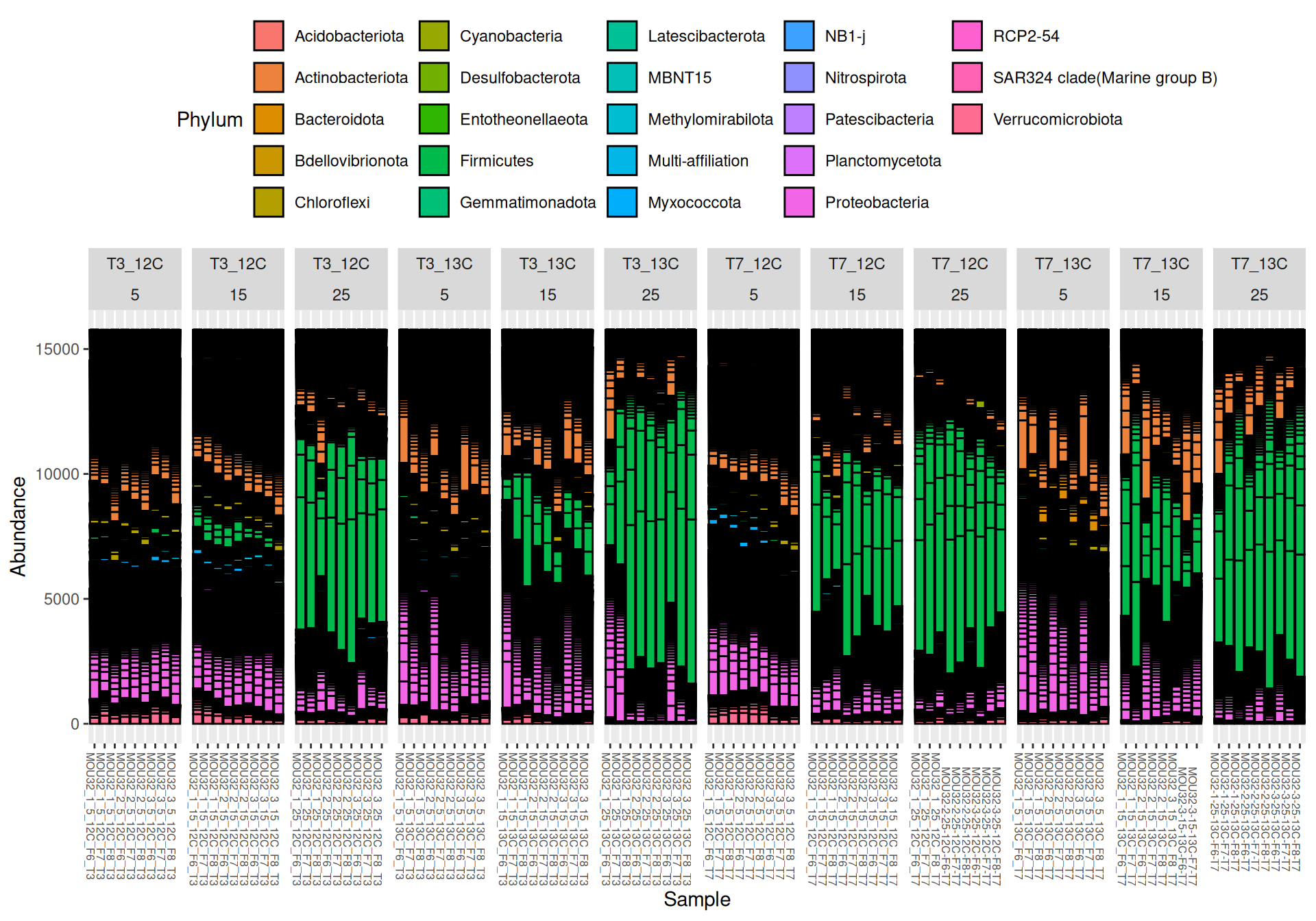
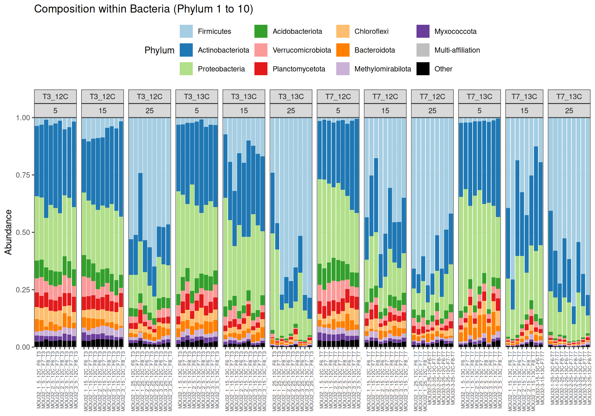
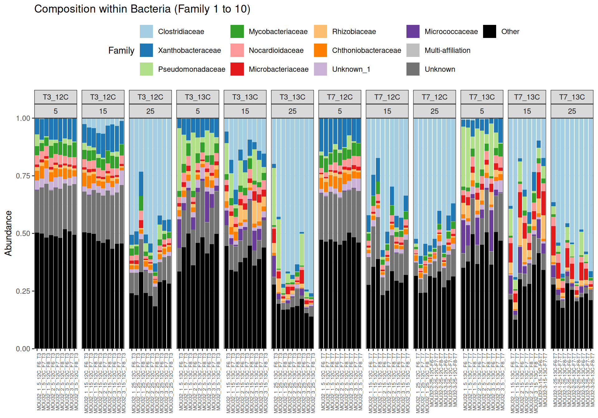
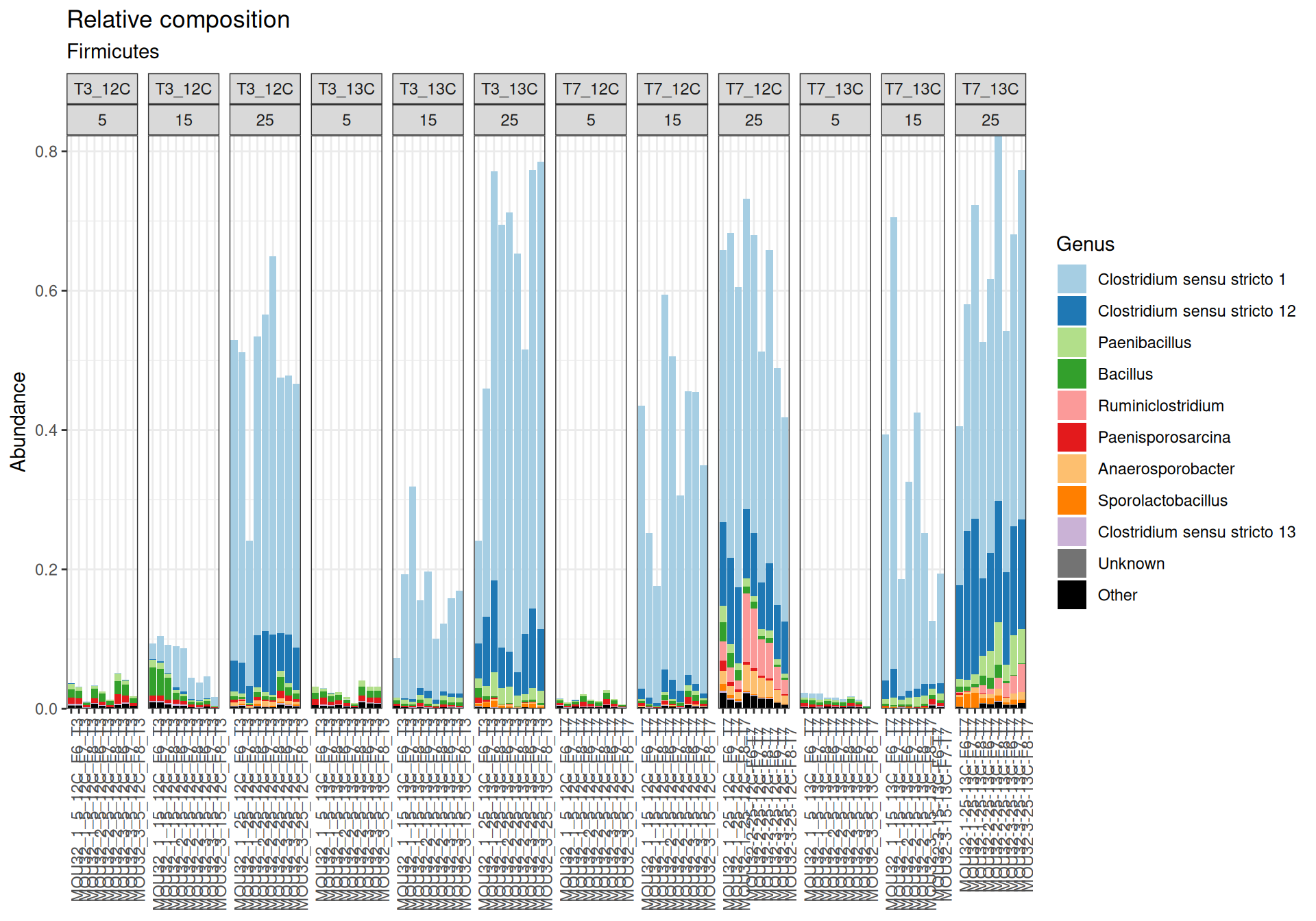
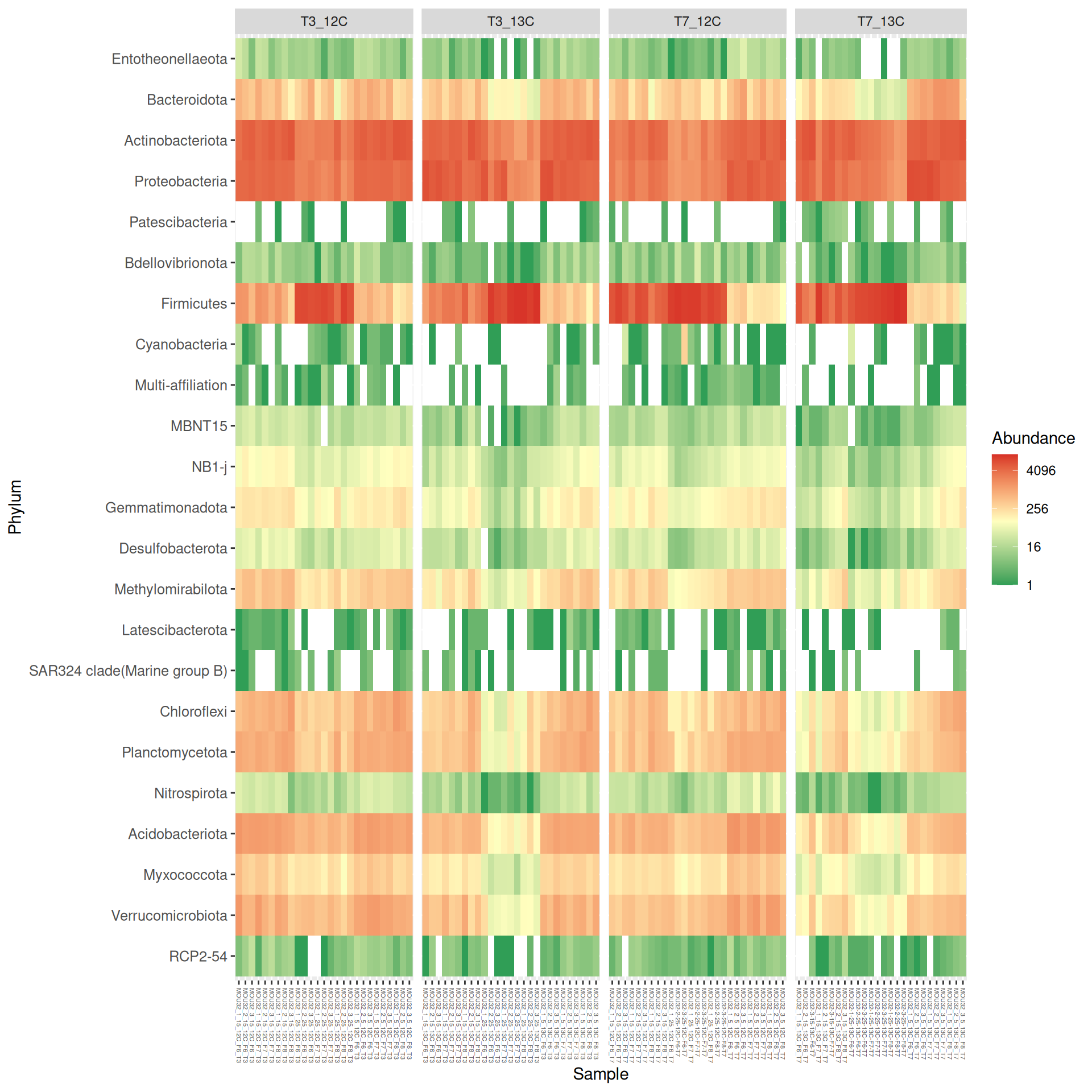
Firmicutes, Actinobacteriota and Proteobacteria are dominants in major samples. Firmicutes appear mainly at Temperature > 15`. Bacteroidota, Methylomirabilota and Myxococcota are few abundants.
Problematic taxa
                   taxa  Kingdom       Phylum       Class           Order
Cluster_209 Cluster_209 Bacteria Bacteroidota Bacteroidia Chitinophagales
Cluster_179 Cluster_179 Bacteria Bacteroidota Bacteroidia    Cytophagales
Cluster_655 Cluster_655 Bacteria Bacteroidota Bacteroidia Chitinophagales
                      Family   Genus rank
Cluster_209 Chitinophagaceae Unknown    2
Cluster_179  Microscillaceae Unknown    3
Cluster_655   Saprospiraceae Unknown    7
Alpha-diversity
Alpha-diversity
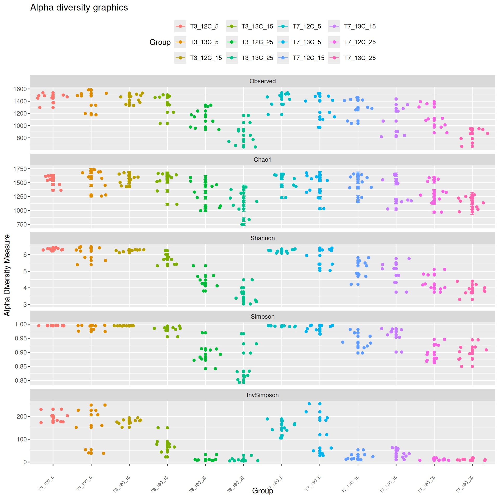
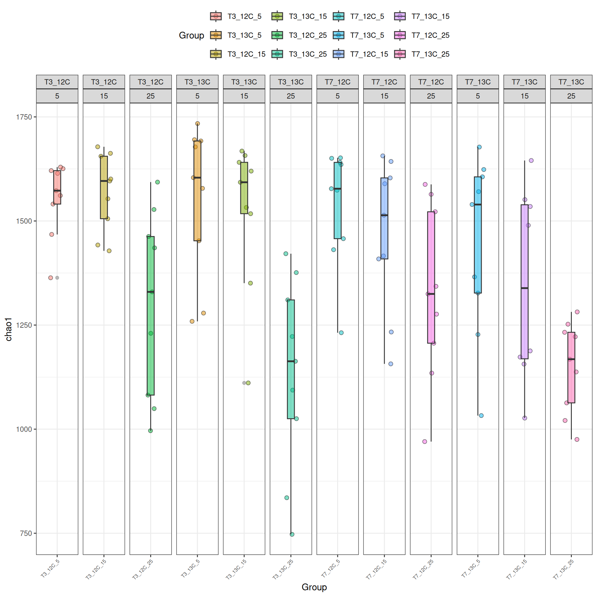
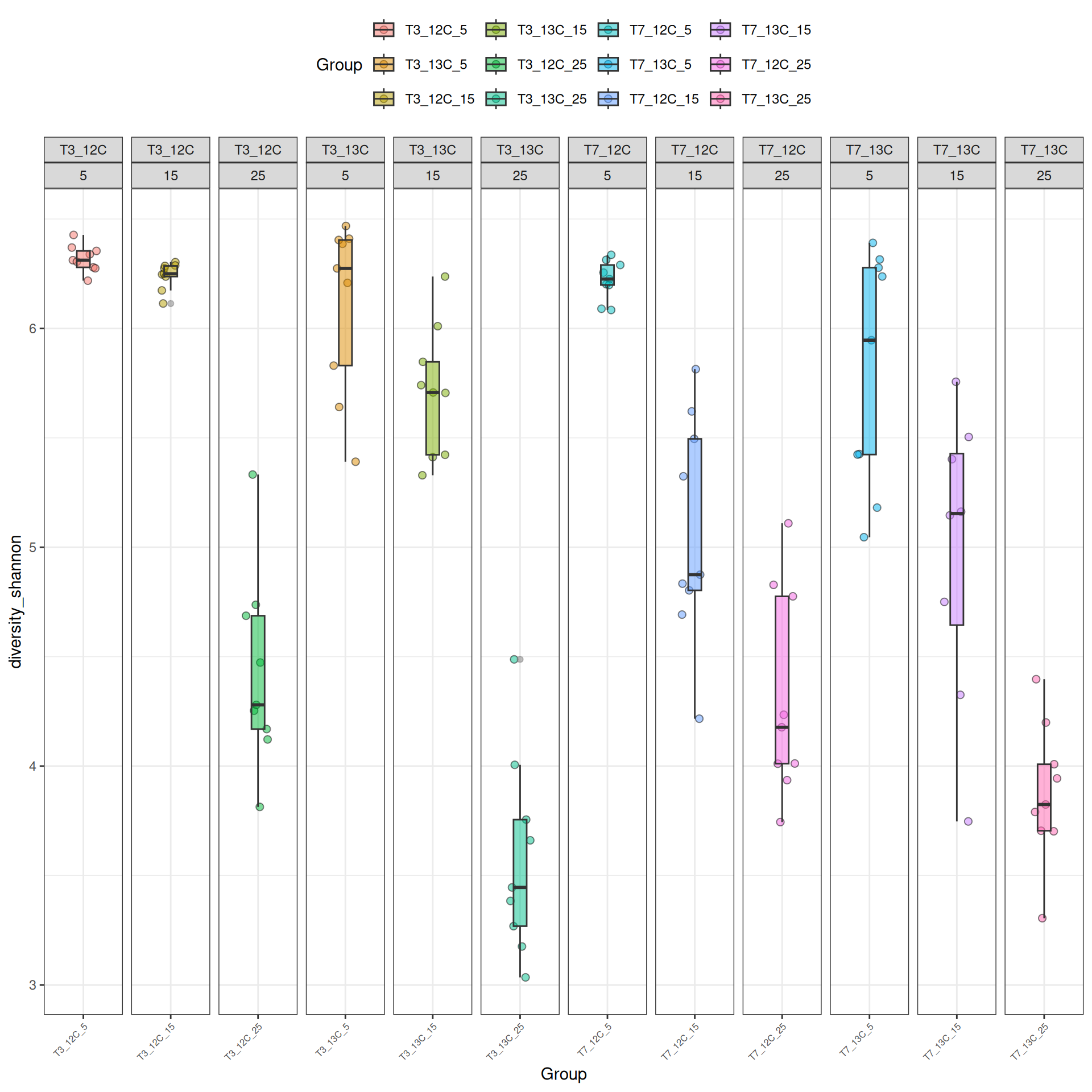
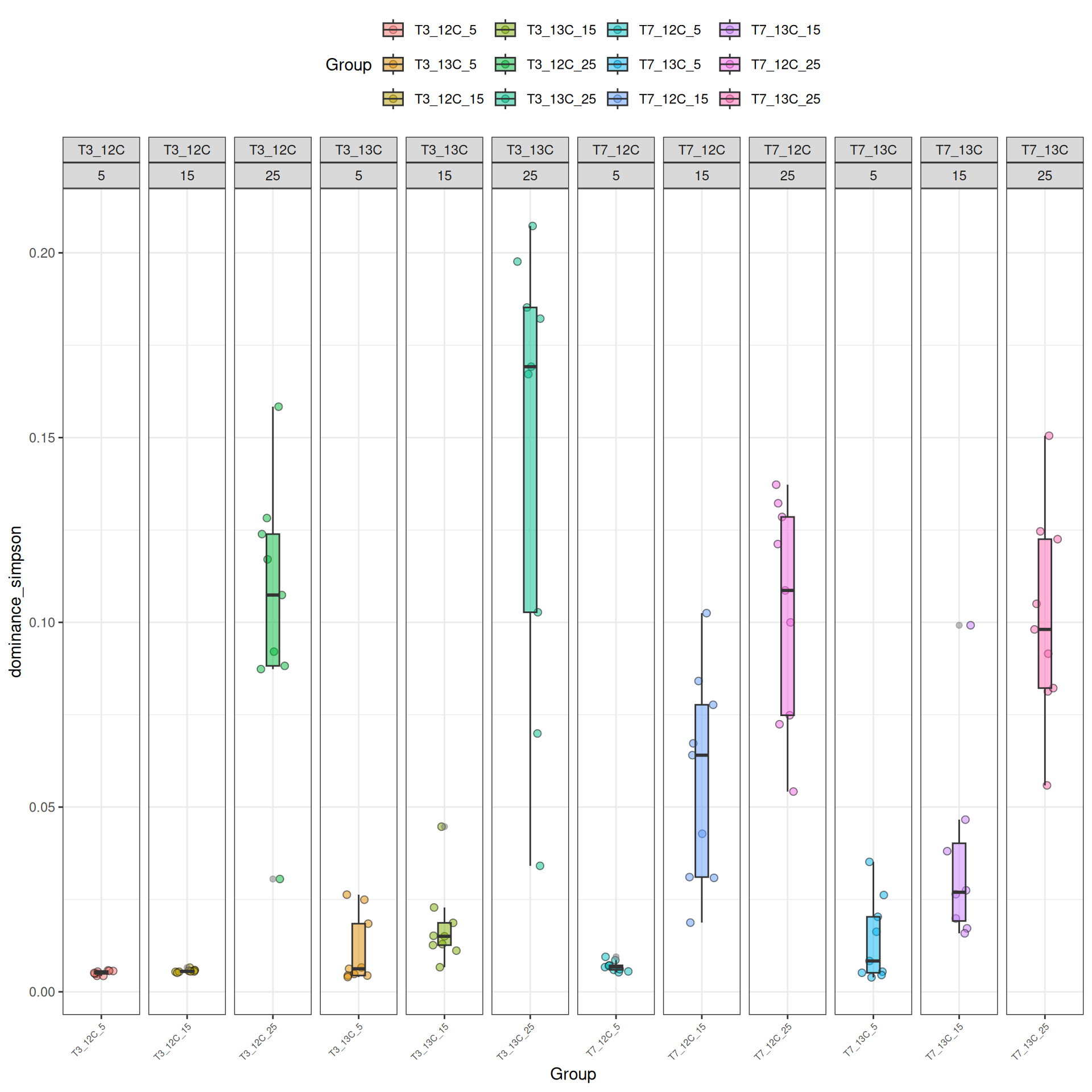
Alpha-diversity represents diversity within a sample (i.e. ecosystem). The most commonly used measures of diversity are : Observed, Chao1, Shannon, and Simpson. Richness (i.e. Observed) is simply the number of species present in the sample and Shannon is another measure based on species richness. Chao1 is an estimator of the number of species applied to the presence/absence data for each species. The Simpson index gives more importance to abundant species.
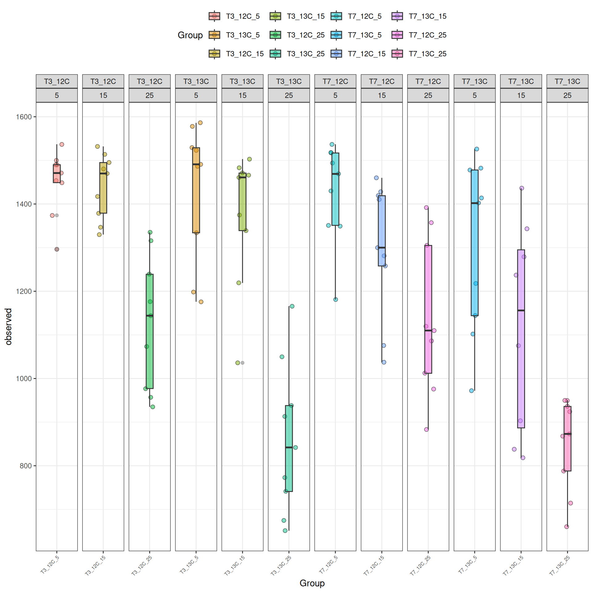
The alpha diversities decrease with Temperature. At Temperature 25, the observed diversity is different between 12C and 13C. Statistical tests are needed to explore the effect of Temperature and Time_Gluc.
Alpha-diversity - statistical tests
We calculated the alpha-diversity indices and combined them with covariates from experimental design. We tested the influence Time_Gluc and Temperature on Observed alpha-diversity.
Richness (Observed diversity) is significantly different between Time_Gluc and Temperature and the interaction.
Show the code
#testsEMM <-emmeans(alphadiv.lm, ~ Time_Gluc*Temperature)# tests correction are performed within the variable# P value adjustment: tukey method for comparingcomp1 <-pairs(EMM, simple ="Time_Gluc")# P value adjustment: tukey method for comparingcomp2 <-pairs(EMM, simple ="Temperature")
Show the code
# P value adjustment: tukey method for comparingres_emm <-contrast(EMM, method ="revpairwise", by =NULL,enhance.levels =c("Time_Gluc", "Temperature"), adjust ="tukey")
Results
Richness (Observed diversity) is significantly different between Time_Gluc for some pairwise comparisons at Temperature 15 and 25 at significance level 0.05. At Temperature = 25, the difference is significative between T3_12C and T3_13C, and also between T7_12C and T7_13C. Richness is significantly different between Temperature for each Time_Gluc level except between Temperature = 5 - Temperature = 15 at Time_Gluc = T7_13C. See the results in the file file.
Description
Excel file containing the results of alpha diversity tests for rarefied samples at T3 and T7.
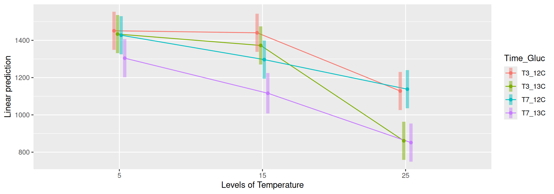
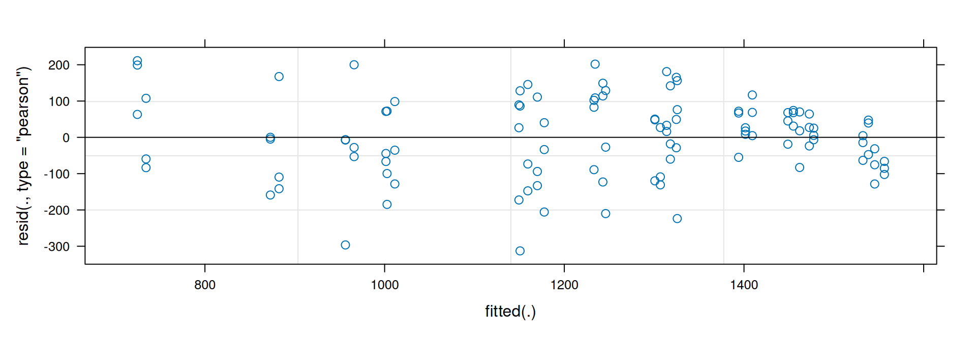
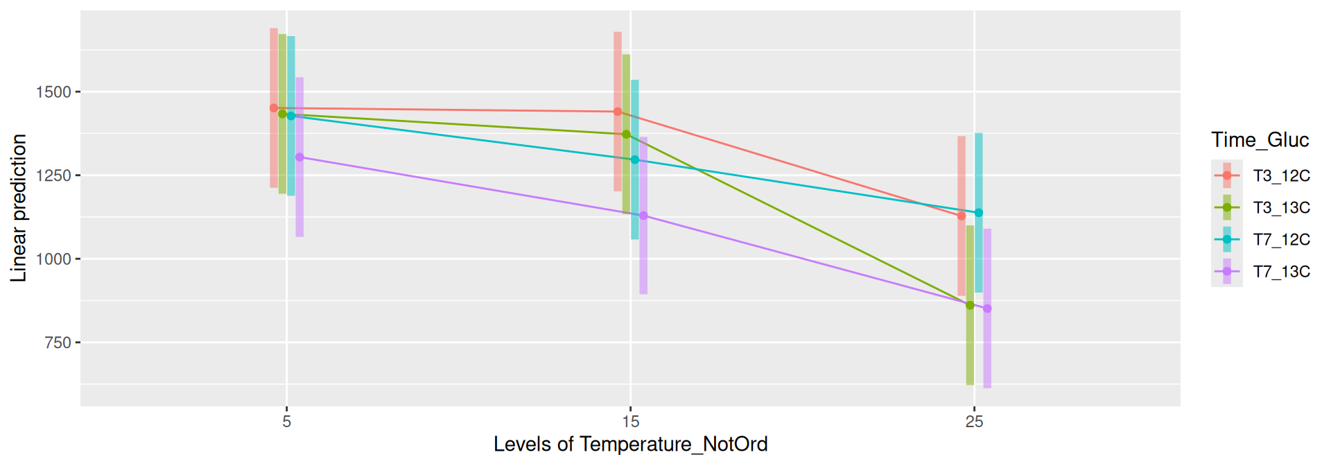
Linear mixed model with interaction
We tested the influence Time_Gluc and Temperature on Observed alpha-diversity. We performed a linear mixed model with Time_Gluc, Temperature and the interaction Time_Gluc x Temperature as fixed effects and FractionOnCsClGradientas a random effect. The random error term depends on each FractionOnCsClGradient for the intercept .
Show the code
# model with only fixed effects # look at the most important factors# alphadiv.aov <- aov(Observed ~ 0 + Time_Gluc*Temperature_NotOrd, data = div_data)# summary(alphadiv.aov)# add a random effect# Note that the ORDER of effects is important# alphadiv.lmer2 <- lmer(Observed ~ 0 + Time_Gluc*Temperature_NotOrd + (1 + Time_Gluc + Temperature_NotOrd | FractionOnCsClGradient), data = div_data)# summary(alphadiv.lmer2)# anova(alphadiv.lmer2)# ranova(alphadiv.lmer2)alphadiv.lmer1 <-lmer(Observed ~0+ Time_Gluc*Temperature_NotOrd + (1| FractionOnCsClGradient), data = div_data)summary(alphadiv.lmer1)
# Test for normality# par(mfrow = c(1, 2))# qqnorm(ranef(alphadiv.lmer1)$FractionOnCsClGradient[,"(Intercept)"], # main = "Random effects")# qqnorm(resid(alphadiv.lmer1), main = "Residuals")# interaction visualisationemmip(alphadiv.lmer1, Time_Gluc ~ Temperature_NotOrd, CIs =TRUE)
Results
Richness (Observed diversity) is significantly different between Time_Gluc and Temperature and the interaction. The random effect FractionOnCsClGradient is significatively different between Intercept but do not depend on Time and Temperature (not shown).
Show the code
#testsEMM <-emmeans(alphadiv.lmer1, ~ Time_Gluc*Temperature_NotOrd)# tests correction are performed within the variable# P value adjustment: tukey method for comparingcomp1 <-pairs(EMM, simple ="Time_Gluc")# P value adjustment: tukey method for comparingcomp2 <-pairs(EMM, simple ="Temperature_NotOrd")
Results
Richness (Observed diversity) is significantly different between Time_Gluc for some pairwise comparisons at each Temperature at significance level 0.05. Richness is significantly different between Temperature for each Time_Gluc level except between Temperature = 5 - Temperature = 15 at Time = T3. See the results in the file file.
Description
Excel file containing the results of alpha diversity tests for rarefied samples at T3 and T7.
Beta-diversity
The dissimilarity between samples based on taxonomic composition is calculated with one of these Beta diversities: Bray-Curtis, Unweighted and weighted Unifrac, Jaccard index. The Jaccard index uses presence/absence information only whereas UniFrac integrates information from the phylogenetic tree.
# Mahendra's functionmy_plot <-function(variable1, variable2, physeq = mydata_rare) { .plot <-function(distance) { .distance <- distance_list[[distance]] %>%as.matrix() %>%`[`(sample_names(physeq), sample_names(physeq)) %>%as.dist() p <-plot_ordination(physeq,ordinate(physeq, method ="MDS", distance = .distance),color = variable1, shape = variable2) +scale_color_brewer(palette ="Paired") +theme(legend.position ="none") +ggtitle(distance)# print(p) } plots <-lapply(names(distance_list), .plot) legend <- cowplot::get_legend(plots[[1]] +theme(legend.position ="bottom")) pgrid <- cowplot::plot_grid(plotlist = plots) cowplot::plot_grid(pgrid, legend, ncol =1, rel_heights =c(1, .1))}# Mahendra's function# used own color's palette and shapemy_plot2 <-function(variable1, variable2, physeq = mydata_rare, shapeval, colorpal) { .plot <-function(distance) { .distance <- distance_list[[distance]] %>%as.matrix() %>%`[`(sample_names(physeq), sample_names(physeq)) %>%as.dist() p <-plot_ordination(physeq,ordinate(physeq, method ="MDS", distance = .distance),color = variable1, shape = variable2) +scale_shape_manual(values = shapeval) +scale_color_manual(name = colorpal$name,labels = colorpal$labels,values = colorpal$values ) +theme(legend.position ="none") +ggtitle(distance)# print(p) } plots <-lapply(names(distance_list), .plot) legend <- cowplot::get_legend(plots[[1]] +theme(legend.position ="bottom")) pgrid <- cowplot::plot_grid(plotlist = plots) cowplot::plot_grid(pgrid, legend, ncol =1, rel_heights =c(1, .1))}# Mahendra's function# used own color's palette and shapemy_pcoa_with_arrows2 <-function(physeq = mydata_rare, variable1, variable2, shapeval, colorpal) {# select samples of interest where all samples were used to calculate the distances between samples # dist.jac is previously calculated with all samples of the study#dist.c <- phyloseq::distance(physeq, "jaccard") dist.c <- dist.bc %>%as.matrix() %>%`[`(sample_names(physeq), sample_names(physeq)) %>%as.dist() ord.c <-ordinate(physeq, "MDS", dist.bc) p <-plot_ordination(physeq, ord.c)# ## Build arrow data plot_data <- p$data arrow_data <- plot_data %>%group_by(pick({{variable2}}, {{variable1}})) %>%arrange({{variable1}}) %>%mutate(xend = Axis.1, xstart =lag(xend),yend = Axis.2, ystart =lag(yend) )## Plot with arrows p +aes(shape = .data[[ variable2 ]], color = .data[[ variable1 ]]) +scale_shape_manual(values = shapeval) +scale_color_manual(name = colorpal$name,labels = colorpal$labels,values = colorpal$values) +theme_bw() +geom_segment(data = arrow_data,aes(x = xstart, y = ystart, xend = xend, yend = yend),linewidth =0.8, linetype ="3131",# arrow = arrow(length=unit(0.1,"inches")),show.legend =FALSE) +geom_point(size =3) +theme(legend.position ="bottom")}
Show the code
# MDS plot for samples of interests # from distance calculated with all samples of the complete study# used https://colorbrewer2.org/#type=qualitative&scheme=Paired&n=12# Time_pal <- list(# name = "Time",# labels = c("T0", "T3", "T7", "T14", "T28"),# values = c("#1f78b4", "#b2df8a", "#984ea3", "#ff7f00", "#a65628")# )Time_Gluc_pal <-list(name ="Time_Gluc",labels =c("T3_12C", "T3_13C", "T7_12C", "T7_13C"),values =c("#b2df8a", "#33a02c", "#cab2d6", "#984ea3"))Temperature_shape <-list(values =c(16,17,15))my_plot2(variable1 ="Time_Gluc",variable2 ="Temperature",physeq = physeq_rare,shapeval = Temperature_shape$values,colorpal = Time_Gluc_pal )
Show the code
# MDS plot for samples of interests # from distance calculated with all samples of the complete study# used https://colorbrewer2.org/#type=qualitative&scheme=Paired&n=12p <-my_pcoa_with_arrows2(variable1 ="Time_Gluc",variable2 ="Temperature",physeq = physeq_rare,shapeval = Temperature_shape$values,colorpal = Time_Gluc_pal)p
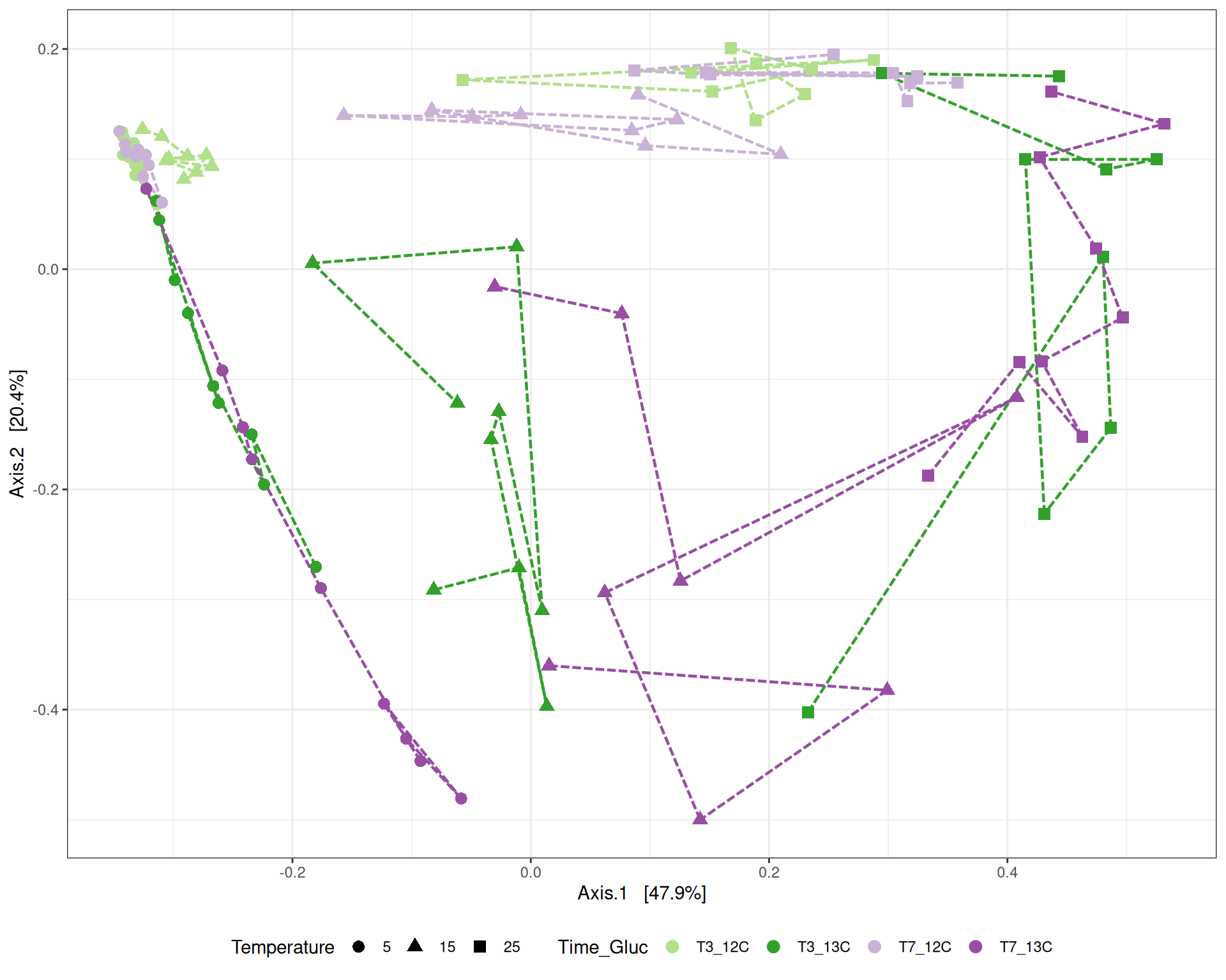
MDS plot
The Multidimensional scaling (MDS / PCoA) based on Bray-Curtis distance showed that samples were distributed according to Time_Gluc and Temperature variables on the first two axes. Differences are more important between Temperature 15 and 25. We observed also differences between 12C and 13C. The variance in community composition is mainly explained by Temperature on the axis 1 and by Glucose on the axis 2.
Beta-diversity - Tests
Show the code
metadata <-sample_data(physeq_rare) %>%as("data.frame")# assess significance for each term sequentially from first to last# importance of the order of the introduced factors in the modelmodel <- vegan::adonis2(dist.bc ~ Temperature*Time_Gluc, data = metadata, permutations =9999, by ="terms")print(model)
Permutation test for adonis under reduced model
Terms added sequentially (first to last)
Permutation: free
Number of permutations: 9999

vegan::adonis2(formula = dist.bc ~ Temperature * Time_Gluc, data = metadata, permutations = 9999, by = "terms")
                       Df SumOfSqs      R2       F Pr(>F)
Temperature             2   7.5330 0.41569 62.4153  1e-04 ***
Time_Gluc               3   3.4981 0.19303 19.3225  1e-04 ***
Temperature:Time_Gluc   6   1.3578 0.07493  3.7501  1e-04 ***
Residual               95   5.7328 0.31635
Total                 106  18.1217 1.00000
---
Signif. codes:  0 '***' 0.001 '**' 0.01 '*' 0.05 '.' 0.1 ' ' 1
Results
The change in microbiota composition measured by the Bray-Curtis Beta diversity is significantly different between Time_Gluc, and Temperature and also between the levels of the interaction factor Time_Gluc:Temperature at 0.05 significance level.
Show the code
par(mar =c(3, 0, 2, 0), cex =0.6)phyloseq.extended::plot_clust(physeq_rare, dist ="bray", method ="ward.D2", color ="Group",title ="Clustering of samples (Bray-Curtis + Ward)")
Results
Hierarchical clustering based on the Bray-Curtis dissimilarity and the Ward aggregation criterion shows that sample composition is not entirely structured by Time_Gluc and Temperature.
At Phylum taxonomic levels, we created heatmap plot using ordination methods to organize the rows.
Family
Show the code
# method = NULL if not ordinationp <- phyloseq::plot_heatmap(tax_glom(physeq_rare, taxrank="Phylum"), method ="MDS",distance ="bray",sample.order="SampleLabel", # not ordination# taxa.order = "Family",taxa.label ="Phylum") +facet_grid(~ Time_Gluc, scales ="free_x", space ="free_x") +scale_fill_gradient2(low ="#1a9850", mid ="#ffffbf", high ="#d73027",na.value ="white", trans = scales::log_trans(4),midpoint =log(100, base =4))p
1. McMurdie PJ, Holmes S. Phyloseq: An r package for reproducible interactive analysis and graphics of microbiome census data. PloS one. 2013;8:e61217.
This document will not be accessible without prior agreement of the partners
A work by Migale Bioinformatics Facility
Université Paris-Saclay, INRAE, MaIAGE, 78350, Jouy-en-Josas, France
Université Paris-Saclay, INRAE, BioinfOmics, MIGALE bioinformatics facility, 78350, Jouy-en-Josas, France
Source Code
---title: "TEMPO"search: falsenavbar: falsesubtitle: "Application of stable isotope probing to identify temperature responsive bacterial taxa at the level of 3-hydroxy fatty acid synthesis: Time T3 and T7"author: - name: Olivier Rué orcid: 0000-0003-1689-0557 email: olivier.rue@inrae.fr affiliations: - name: Migale bioinformatics facility adress: Domaine de Vilvert city: Jouy-en-Josas state: France - name: Christelle Hennequet-Antier orcid: 0000-0001-5836-2803 email: christelle.hennequet-antier@inrae.fr affiliations: - name: Migale bioinformatics facility adress: Domaine de Vilvert city: Jouy-en-Josas state: Francedate: "2023-11-22"date-modified: todaycategories: [in progress, collaboration]image: "preview.jpg"reader-mode: falsefig-cap-location: bottomtbl-cap-location: toplicense: "This document will not be accessible without prior agreement of the partners"format: html: embed-resources: false toc: true toc-location: right page-layout: article code-fold: true code-summary: "Show the code" code-tools: true code-overflow: wraplightbox: auto---```{r setup, include=FALSE}knitr::opts_chunk$set(eval=TRUE, echo =TRUE, cache = FALSE, message = FALSE, warning = FALSE, cache.lazy = FALSE, fig.height = 3.5, fig.width = 10)``````{r load-packages, echo=FALSE, eval=TRUE, cache = FALSE}library(DT)library(scales)library(tidyverse)library(kableExtra)library(phyloseq)library(phyloseq.extended)library(data.table)library(InraeThemes)library(MicrobiotaProcess)library(metacoder) #visualization and annotation of phylogenetic treeslibrary(ggtree) #visualization and annotation of phylogenetic treeslibrary(ggtreeExtra) #visualization and annotation of phylogenetic treeslibrary(emmeans)#post hoc testslibrary(lme4) # linear mixed modelslibrary(lmerTest) # add pvalues testslibrary(openxlsx) #save results to excel sheetslibrary(mia) # microbiome analysis with SummarizedExperiment and TreeSummarizedExperimentlibrary(ComplexHeatmap) # produce heatmaplibrary(viridis)``````{r datatable global options, echo=FALSE, eval=TRUE}options(DT.options = list(pageLength = 10, scrollX = TRUE, language = list(search = 'Filter:'), dom = 'lftipB', buttons = c('copy', 'csv', 'excel')))```{{< include /resources/_includes/_intro_note.qmd >}}# Aim of the projectThe aim of the project is to provide a better understanding of how soil bacteria respond to temperature variations at the membrane level. Bacterial lipids can be used in paleoclimatology to reconstruct temperature of past climates in marine and terrestrial archives. This involves the use of proxies and calculations that are based on the relative amounts of these lipids. In soil, only one organic proxy is available, mainly due to the difficulty to work on soil, which is much more heterogeneous in structure than aquatic environments. A drawback of this sungle proxy is the error which is associated with it as well as the lack of confirmation of the result by a different approach. A new proxy based on 3-hydroxy fatty acids has been proposed in 2016. To better understand and validate this proxy, as well as to investigate new more precise proxies, we aim at understanding what soil bacterial species contribute to the proposed proxy by investigating their response te temperature at the taxonomic and lipid levels. We have used a DNA- and lipid-SIP approach during a time-course experiment and are now at the stage of analyzing what species have used the 13C labelled substrate in a temperature dependent manner. The profile of the enriched taxa in the 13C fraction will be compared in the different samples (different temperature, different incubation time) and will be compared with the 13C-enriched lipid profiles in the same samples.## Partners* Olivier Rué - Migale bioinformatics facility - BioInfomics - INRAE* Christelle Hennequet-Antier - Migale bioinformatics facility - BioInfomics - INRAE* Sylvie Collin - Sorbonne Université## DeliverablesDeliverables agreed at the preliminary meeting (@tbl-deliverables).| | Definition ||------|------|| 1 | HTML report |: Deliverables {#tbl-deliverables}# Data management{{< include /resources/_includes/_data_management.qmd >}}# Biostatistics{{< include /resources/_includes/_phyloseq.qmd >}}The available metadata are:<!-- ```{r} --><!-- metadata <- read.table("data/metadata.tsv", row.names = 1, header = TRUE, sep = "\t", stringsAsFactors = FALSE) --><!-- metadata <- metadata %>% --><!-- mutate(Time = as.factor(Time)) %>% --><!-- mutate(Temperature = as.factor(Temperature)) %>% --><!-- mutate(SampleID = as.character(SampleID)) --><!-- metadata %>% --><!-- datatable() --><!-- ``` -->```{r}metadata <-read_tsv("../data/metadata.tsv", col_types =cols(SampleName =col_character(), Time =col_factor(levels =c("T0", "T3", "T7", "T14", "T28"), ordered =TRUE), Temperature =col_factor(levels =c("5", "15", "25"), ordered =TRUE),Replicate =col_factor(levels =c("1", "2", "3"), ordered =TRUE) )) %>%column_to_rownames(var="SampleName")metadata <- metadata %>%mutate(Temperature_NotOrd =factor(Temperature, levels =c("5", "15", "25"), ordered =FALSE)) %>%mutate(Time_Gluc =case_when( Time =="T3"~paste(Time, Glucose, sep="_"), Time =="T7"~paste(Time, Glucose, sep="_"),.default = Time )) %>%mutate(Time_Gluc =factor(Time_Gluc,levels =c("T0", "T3_12C", "T3_13C", "T7_12C", "T7_13C", "T14", "T28"))) %>%mutate(Group =paste(Time_Gluc, Temperature, sep="_")) %>%mutate(Group =factor(Group, levels =c("T0_5", "T0_15", "T0_25", "T3_12C_5", "T3_13C_5", "T3_12C_15", "T3_13C_15", "T3_12C_25", "T3_13C_25", "T7_12C_5", "T7_13C_5", "T7_12C_15", "T7_13C_15", "T7_12C_25", "T7_13C_25", "T14_5", "T14_15", "T14_25", "T28_5", "T28_15", "T28_25")) ) %>%mutate(SampleLabel =case_when(is.na(FractionOnCsClGradient) ==TRUE~paste(Group, Replicate, sep="_"),.default =paste(Group, FractionOnCsClGradient, Replicate, sep="_")))#spec(metadata)# metadata %>% # datatable()``````{r}biomfile <-paste0("../html/","affiliation.biom")physeq <-import_frogs(biomfile, taxMethod ="blast")sample_data(physeq) <- metadataphy_tree(physeq) <- phyloseq::read_tree("../html/tree.nwk")physeq <- physeq %>% microViz::ps_arrange(Time_Gluc, Temperature, FractionOnCsClGradient)# visualisation and savemetadata %>%datatable()microbiome::summarize_phyloseq(physeq)saveRDS(object = physeq, file="physeq.rds")``````{r}#| label: checkdesign# count number of samples per conditionsample_data(physeq) %>%as_tibble() %>% dplyr::count(Time) sample_data(physeq) %>%as_tibble() %>% dplyr::add_count(Time, Temperature, Glucose) %>% dplyr::select(Time, Temperature, , Glucose, Group, n) %>%distinct() %>%ggplot(., aes(x = Group, y = n, fill = Time)) +geom_bar(stat ="identity") +labs(title="Number of replicates", y ="n") +theme(axis.title.x =element_blank(),axis.text.x =element_text(angle =90, size =8, hjust =1))# frequencies#microbiome::plot_frequencies(sample_data(physeq), "Time", "Group")```:::{.callout-note icon=false}For analysis purposes, the variable `Time_Gluc` is created as the combination of the `Time` and `Glucose` variables.:::## Select samples from Time T3 and T7```{r}physeq <- physeq %>% microViz::ps_filter(Time %in%c("T3", "T7")) ```## Rarefaction{{< include /resources/_includes/_rarefaction.qmd >}}::: {.panel-tabset}### Before rarefaction```{r}#| label: plot_bar#| fig-height: 7phyloseq::plot_bar(physeq, x ="SampleLabel", fill ="Phylum") +facet_grid(~ Time_Gluc + Temperature, scales ="free_x", space ="free") +# facet_grid(~Time + Temperature + Glucose, scales = "free_x", space = "free") +theme(axis.text.x =element_text(size =6, hjust =1)) +theme(legend.position="top")``````{r}# sample_sums(physeq) %>% sort() %>% head(n=5)# remove samples with less than nbreads_threshold nbreads_threshold <-11000sample_sums(physeq)[!sample_sums(physeq) > nbreads_threshold]physeq <- microViz::ps_filter(physeq, sample_sums(physeq) > nbreads_threshold)``````{r}ggrare(physeq = physeq, step =500, se =FALSE, color ="Group", plot =FALSE, label ="SampleLabel", verbose =FALSE) +# scale_colour_manual(values = group_pal) +geom_vline(xintercept =c(min(sample_sums(physeq))), color ="gray60") +ggtitle("Rarefaction curves")```### After rarefaction```{r}#| label: rarefyphyseq_rare <- phyloseq::rarefy_even_depth(physeq, rngseed =2002, replace =TRUE)``````{r}#| label: plot_bar_rare#| fig-height: 7phyloseq::plot_bar(physeq_rare, fill="Phylum") +facet_grid(~ Time_Gluc + Temperature, scales ="free_x", space ="free") +theme(axis.text.x =element_text(size =6, hjust =1)) +theme(legend.position="top")```::::::{.callout-important icon=false}# ResultsOne sample was removed due to a low number of reads, less than `r as.integer(nbreads_threshold)`.After rarefaction, all depths are equal to `r as.integer(min(phyloseq::sample_sums(physeq)))`. The dataset contains `r as.integer(sum(phyloseq::sample_sums(physeq_rare)))` sequences allocated to `r as.integer(phyloseq::ntaxa(physeq_rare))` taxa and `r as.integer(phyloseq::nsamples(physeq_rare))` samples. :::## Taxonomic composition```{r}#| fig-height: 7phyloseq.extended::plot_composition(physeq = physeq_rare, taxaRank1 ="Kingdom", taxaSet1 ="Bacteria", taxaRank2 ="Phylum", numberOfTaxa =10L) +facet_grid(~ Time_Gluc + Temperature, scales ="free_x", space ="free") +theme(axis.text.x =element_text(size =6, hjust =1)) +theme(legend.position="top")``````{r}#| fig-height: 7phyloseq.extended::plot_composition(physeq = physeq_rare, taxaRank1 ="Kingdom", taxaSet1 ="Bacteria", taxaRank2 ="Family", numberOfTaxa =10L) +facet_grid(~ Time_Gluc + Temperature, scales ="free_x", space ="free") +theme(axis.text.x =element_text(size =6, hjust =1)) +theme(legend.position="top")```::: {.callout-important icon=false}# ResultsFirmicutes, Actinobacteriota and Proteobacteria are dominants in major samples. Firmicutes appear mainly at ` `Temperature > 15`. Bacteroidota, Methylomirabilota and Myxococcota are few abundants.:::Focus on the genus rank across these major phyla.::: {.panel-tabset}### Actinobacteriota ```{r}#| fig-height: 7phyloseq.extended::plot_composition(physeq = physeq_rare, taxaRank1 ="Phylum", taxaSet1 ="Actinobacteriota", taxaRank2 ="Genus") +facet_grid( ~ Time_Gluc + Temperature, scales ="free_x", space ="free_x") +labs(title ="Relative composition", subtitle ="Actinobacteriota")```### Proteobateria ```{r}#| fig-height: 7phyloseq.extended::plot_composition(physeq = physeq_rare, taxaRank1 ="Phylum", taxaSet1 ="Proteobacteria", taxaRank2 ="Genus") +facet_grid( ~ Time_Gluc + Temperature, scales ="free_x", space ="free_x") +labs(title ="Relative composition", subtitle ="Proteobacteria")```### Firmicutes ```{r}#| fig-height: 7phyloseq.extended::plot_composition(physeq = physeq_rare, taxaRank1 ="Phylum", taxaSet1 ="Firmicutes", taxaRank2 ="Genus") +facet_grid( ~ Time_Gluc + Temperature, scales ="free_x", space ="free_x") +labs(title ="Relative composition", subtitle ="Firmicutes")```### Bacteroidota ```{r}#| fig-height: 7phyloseq.extended::plot_composition(physeq = physeq_rare, taxaRank1 ="Phylum", taxaSet1 ="Bacteroidota", taxaRank2 ="Genus") +facet_grid( ~ Time_Gluc + Temperature, scales ="free_x", space ="free_x") +labs(title ="Relative composition", subtitle ="Bacteroidota")```:::## Alpha-diversity::: {.callout-note icon=false}# Alpha-diversityAlpha-diversity represents diversity within a sample (i.e. ecosystem). The most commonly used measures of diversity are : Observed, Chao1, Shannon, and Simpson. Richness (i.e. Observed) is simply the number of species present in the sample and Shannon is another measure based on species richness. Chao1 is an estimator of the number of species applied to the presence/absence data for each species. The Simpson index gives more importance to abundant species.:::::: {.panel-tabset}### ALL indexes```{r}#| label: alpha_diversity_all#| fig-height: 10# plot alpha diversityphyloseq::plot_richness(physeq = physeq_rare, x ="Group", color="Group", title ="Alpha diversity graphics", measures =c("Observed", "Chao1", "Shannon", "Simpson", "InvSimpson"), nrow=5) +geom_jitter() +scale_fill_brewer(palette ="Paired") +theme(axis.text.x =element_text(size =6, angle =45, hjust =1)) +theme(legend.position="top")```### Observed```{r}#| label: alpha_diversity_obs1#| fig-height: 10# plot alpha diversity p.alphadiversity <- microbiome::boxplot_alpha(physeq_rare, index =c("Observed"),x_var ="Group", )p.alphadiversity +facet_grid(cols =vars(Time_Gluc, Temperature), scales ="free_x", space ="free_x") +theme(axis.text.x =element_text(size =6, angle =45, hjust =1)) +theme(legend.position="top")```### Chao1```{r}#| label: alpha_diversity_Chao1#| fig-height: 10# plot alpha diversity p.alphadiversity <- microbiome::boxplot_alpha(physeq_rare, index =c("Chao1"),x_var ="Group", )p.alphadiversity +facet_grid(cols =vars(Time_Gluc, Temperature), scales ="free_x", space ="free_x") +theme(axis.text.x =element_text(size =6, angle =45, hjust =1)) +theme(legend.position="top")```### Shannon```{r}#| label: alpha_diversity_Shannon#| fig-height: 10# plot alpha diversity p.alphadiversity <- microbiome::boxplot_alpha(physeq_rare, index =c("Shannon"),x_var ="Group", )p.alphadiversity +facet_grid(cols =vars(Time_Gluc, Temperature), scales ="free_x", space ="free_x") +theme(axis.text.x =element_text(size =6, angle =45, hjust =1)) +theme(legend.position="top")```### Simpson```{r}#| label: alpha_diversity_Simpson#| fig-height: 10# plot alpha diversity p.alphadiversity <- microbiome::boxplot_alpha(physeq_rare, index =c("Simpson"),x_var ="Group", )p.alphadiversity +facet_grid(cols =vars(Time_Gluc, Temperature), scales ="free_x", space ="free_x") +theme(axis.text.x =element_text(size =6, angle =45, hjust =1)) +theme(legend.position="top")```:::::: {.callout-important icon=false}# ResultsThe alpha diversities decrease with `Temperature`. At `Temperature 25`, the observed diversity is different between `12C` and `13C`. Statistical tests are needed to explore the effect of `Temperature` and `Time_Gluc`.:::## Alpha-diversity - statistical testsWe calculated the alpha-diversity indices and combined them with covariates from experimental design. We tested the influence `Time_Gluc` and `Temperature` on Observed alpha-diversity.```{r}#| label: alpha_div_covariatesdiv_data <-cbind(estimate_richness(physeq_rare), ## diversity indicessample_data(physeq_rare) ## covariates )```<!-- MODIF Test sans effet aléatoire -->We tested the influence `Time_Gluc` and `Temperature` on `Observed` alpha-diversity.```{r}#| label: posthoc_alpha_divalphadiv.lm <-lm(Observed ~ Time_Gluc*Temperature, data = div_data)anova(alphadiv.lm)# interaction visualisationemmip(alphadiv.lm, Time_Gluc ~ Temperature, CIs =TRUE)```::: {.callout-important icon=false}# ResultsRichness (Observed diversity) is significantly different between `Time_Gluc` and `Temperature` and the interaction.:::```{r}#testsEMM <-emmeans(alphadiv.lm, ~ Time_Gluc*Temperature)# tests correction are performed within the variable# P value adjustment: tukey method for comparingcomp1 <-pairs(EMM, simple ="Time_Gluc")# P value adjustment: tukey method for comparingcomp2 <-pairs(EMM, simple ="Temperature")``````{r}#| label: dataframe_allcontrast# P value adjustment: tukey method for comparingres_emm <-contrast(EMM, method ="revpairwise", by =NULL,enhance.levels =c("Time_Gluc", "Temperature"), adjust ="tukey")``````{r}#| label: save_allcontrast#| echo: false# using openxlsx package to export resultsexcelsheets <-list(All = res_emm,compbyTime_Gluc = comp1,compbyTemperature = comp2)write.xlsx(excelsheets,file =paste0("comparisons_alpha_diversity_T3-T7_LM", ".xlsx"))```::: {.callout-important icon=false}# ResultsRichness (Observed diversity) is significantly different between `Time_Gluc` for some pairwise comparisons at `Temperature` 15 and 25 at significance level 0.05. At `Temperature = 25`, the difference is significative between `T3_12C` and `T3_13C`, and also between `T7_12C` and `T7_13C`.Richness is significantly different between `Temperature` for each `Time_Gluc` level except between `Temperature = 5 - Temperature = 15` at `Time_Gluc = T7_13C`. See the results in the file file.:::| | Description ||------|------|| {{< downloadthis comparisons_alpha_diversity_T3-T7_LM.xlsx >}} | Excel file containing the results of alpha diversity tests for rarefied samples at T3 and T7. |<!-- FIN MODIF Test sans effet aléatoire -->### Linear mixed model with interactionWe tested the influence `Time_Gluc` and `Temperature` on `Observed` alpha-diversity. We performed a linear mixed model with `Time_Gluc`, `Temperature` and the interaction `Time_Gluc x Temperature` as fixed effects and `FractionOnCsClGradient`as a random effect. The random error term depends on each `FractionOnCsClGradient` for the intercept .```{r}# model with only fixed effects # look at the most important factors# alphadiv.aov <- aov(Observed ~ 0 + Time_Gluc*Temperature_NotOrd, data = div_data)# summary(alphadiv.aov)# add a random effect# Note that the ORDER of effects is important# alphadiv.lmer2 <- lmer(Observed ~ 0 + Time_Gluc*Temperature_NotOrd + (1 + Time_Gluc + Temperature_NotOrd | FractionOnCsClGradient), data = div_data)# summary(alphadiv.lmer2)# anova(alphadiv.lmer2)# ranova(alphadiv.lmer2)alphadiv.lmer1 <-lmer(Observed ~0+ Time_Gluc*Temperature_NotOrd + (1| FractionOnCsClGradient), data = div_data)summary(alphadiv.lmer1)anova(alphadiv.lmer1)ranova(alphadiv.lmer1)plot(alphadiv.lmer1)# Test for normality# par(mfrow = c(1, 2))# qqnorm(ranef(alphadiv.lmer1)$FractionOnCsClGradient[,"(Intercept)"], # main = "Random effects")# qqnorm(resid(alphadiv.lmer1), main = "Residuals")# interaction visualisationemmip(alphadiv.lmer1, Time_Gluc ~ Temperature_NotOrd, CIs =TRUE)```::: {.callout-important icon=false}# ResultsRichness (Observed diversity) is significantly different between `Time_Gluc` and `Temperature` and the interaction. The random effect `FractionOnCsClGradient` is significatively different between `Intercept` but do not depend on `Time` and `Temperature` (not shown).:::```{r}#testsEMM <-emmeans(alphadiv.lmer1, ~ Time_Gluc*Temperature_NotOrd)# tests correction are performed within the variable# P value adjustment: tukey method for comparingcomp1 <-pairs(EMM, simple ="Time_Gluc")# P value adjustment: tukey method for comparingcomp2 <-pairs(EMM, simple ="Temperature_NotOrd")``````{r}#| label: save_allcontrastmixed#| echo: false# using openxlsx package to export resultsexcelsheets <-list(compbyTime = comp1,compbyTemperature = comp2)write.xlsx(excelsheets,file =paste0("comparisons_alpha_diversity_T3-T7_LMMixed", ".xlsx"))```::: {.callout-important icon=false}# ResultsRichness (Observed diversity) is significantly different between `Time_Gluc` for some pairwise comparisons at each `Temperature` at significance level 0.05. Richness is significantly different between `Temperature` for each `Time_Gluc` level except between `Temperature = 5 - Temperature = 15` at `Time = T3`. See the results in the file file.:::| | Description ||------|------|| {{< downloadthis comparisons_alpha_diversity_T3-T7_LMMixed.xlsx >}} | Excel file containing the results of alpha diversity tests for rarefied samples at T3 and T7. |## Beta-diversityThe dissimilarity between samples based on taxonomic composition is calculated with one of these Beta diversities: Bray-Curtis, Unweighted and weighted Unifrac, Jaccard index. The Jaccard index uses presence/absence information only whereas UniFrac integrates information from the phylogenetic tree.<!-- https://microbiome.github.io/OMA/microbiome-diversity.html -->```{r}#| label: distance_betadivdist.jac <- phyloseq::distance(physeq_rare, method ="cc")dist.bc <- phyloseq::distance(physeq_rare, method ="bray")dist.uf <- phyloseq::distance(physeq_rare, method ="unifrac")dist.wuf <- phyloseq::distance(physeq_rare, method ="wunifrac")distance_list <-list("Jaccard"= dist.jac,"Bray-Curtis"= dist.bc,"UniFrac"= dist.uf,"wUniFrac"= dist.wuf)``````{r}#| label: function_cowplot_MDS#| echo: true# Mahendra's functionmy_plot <-function(variable1, variable2, physeq = mydata_rare) { .plot <-function(distance) { .distance <- distance_list[[distance]] %>%as.matrix() %>%`[`(sample_names(physeq), sample_names(physeq)) %>%as.dist() p <-plot_ordination(physeq,ordinate(physeq, method ="MDS", distance = .distance),color = variable1, shape = variable2) +scale_color_brewer(palette ="Paired") +theme(legend.position ="none") +ggtitle(distance)# print(p) } plots <-lapply(names(distance_list), .plot) legend <- cowplot::get_legend(plots[[1]] +theme(legend.position ="bottom")) pgrid <- cowplot::plot_grid(plotlist = plots) cowplot::plot_grid(pgrid, legend, ncol =1, rel_heights =c(1, .1))}# Mahendra's function# used own color's palette and shapemy_plot2 <-function(variable1, variable2, physeq = mydata_rare, shapeval, colorpal) { .plot <-function(distance) { .distance <- distance_list[[distance]] %>%as.matrix() %>%`[`(sample_names(physeq), sample_names(physeq)) %>%as.dist() p <-plot_ordination(physeq,ordinate(physeq, method ="MDS", distance = .distance),color = variable1, shape = variable2) +scale_shape_manual(values = shapeval) +scale_color_manual(name = colorpal$name,labels = colorpal$labels,values = colorpal$values ) +theme(legend.position ="none") +ggtitle(distance)# print(p) } plots <-lapply(names(distance_list), .plot) legend <- cowplot::get_legend(plots[[1]] +theme(legend.position ="bottom")) pgrid <- cowplot::plot_grid(plotlist = plots) cowplot::plot_grid(pgrid, legend, ncol =1, rel_heights =c(1, .1))}# Mahendra's function# used own color's palette and shapemy_pcoa_with_arrows2 <-function(physeq = mydata_rare, variable1, variable2, shapeval, colorpal) {# select samples of interest where all samples were used to calculate the distances between samples # dist.jac is previously calculated with all samples of the study#dist.c <- phyloseq::distance(physeq, "jaccard") dist.c <- dist.bc %>%as.matrix() %>%`[`(sample_names(physeq), sample_names(physeq)) %>%as.dist() ord.c <-ordinate(physeq, "MDS", dist.bc) p <-plot_ordination(physeq, ord.c)# ## Build arrow data plot_data <- p$data arrow_data <- plot_data %>%group_by(pick({{variable2}}, {{variable1}})) %>%arrange({{variable1}}) %>%mutate(xend = Axis.1, xstart =lag(xend),yend = Axis.2, ystart =lag(yend) )## Plot with arrows p +aes(shape = .data[[ variable2 ]], color = .data[[ variable1 ]]) +scale_shape_manual(values = shapeval) +scale_color_manual(name = colorpal$name,labels = colorpal$labels,values = colorpal$values) +theme_bw() +geom_segment(data = arrow_data,aes(x = xstart, y = ystart, xend = xend, yend = yend),linewidth =0.8, linetype ="3131",# arrow = arrow(length=unit(0.1,"inches")),show.legend =FALSE) +geom_point(size =3) +theme(legend.position ="bottom")}```<!-- ```{r} --><!-- #| label: MDS_plot --><!-- #| fig-height: 6 --><!-- my_plot(variable1 = "Time", variable2 = "Temperature", physeq = physeq_rare) --><!-- ``` -->```{r}#| fig-height: 8# MDS plot for samples of interests # from distance calculated with all samples of the complete study# used https://colorbrewer2.org/#type=qualitative&scheme=Paired&n=12# Time_pal <- list(# name = "Time",# labels = c("T0", "T3", "T7", "T14", "T28"),# values = c("#1f78b4", "#b2df8a", "#984ea3", "#ff7f00", "#a65628")# )Time_Gluc_pal <-list(name ="Time_Gluc",labels =c("T3_12C", "T3_13C", "T7_12C", "T7_13C"),values =c("#b2df8a", "#33a02c", "#cab2d6", "#984ea3"))Temperature_shape <-list(values =c(16,17,15))my_plot2(variable1 ="Time_Gluc",variable2 ="Temperature",physeq = physeq_rare,shapeval = Temperature_shape$values,colorpal = Time_Gluc_pal )``````{r}#| fig-height: 8# MDS plot for samples of interests # from distance calculated with all samples of the complete study# used https://colorbrewer2.org/#type=qualitative&scheme=Paired&n=12p <-my_pcoa_with_arrows2(variable1 ="Time_Gluc",variable2 ="Temperature",physeq = physeq_rare,shapeval = Temperature_shape$values,colorpal = Time_Gluc_pal)p```::: {.callout-important icon=false}# MDS plotThe Multidimensional scaling (MDS / PCoA) based on Bray-Curtis distance showed that samples were distributed according to `Time_Gluc` and `Temperature` variables on the first two axes. Differences are more important between `Temperature` 15 and 25. We observed also differences between `12C` and `13C`. The variance in community composition is mainly explained by `Temperature ` on the axis 1 and by `Glucose` on the axis 2. :::## Beta-diversity - Tests```{r}#| label: adonis#| warning: falsemetadata <-sample_data(physeq_rare) %>%as("data.frame")# assess significance for each term sequentially from first to last# importance of the order of the introduced factors in the modelmodel <- vegan::adonis2(dist.bc ~ Temperature*Time_Gluc, data = metadata, permutations =9999, by ="terms")print(model)```::: {.callout-important icon=false}# ResultsThe change in microbiota composition measured by the `Bray-Curtis` Beta diversity is significantly different between `Time_Gluc`, and `Temperature` and also between the levels of the interaction factor `Time_Gluc:Temperature` at 0.05 significance level. :::```{r}#| label: clustering_samplespar(mar =c(3, 0, 2, 0), cex =0.6)phyloseq.extended::plot_clust(physeq_rare, dist ="bray", method ="ward.D2", color ="Group",title ="Clustering of samples (Bray-Curtis + Ward)")```::: {.callout-important icon=false}# ResultsHierarchical clustering based on the `Bray-Curtis` dissimilarity and the `Ward` aggregation criterion shows that sample composition is not entirely structured by `Time_Gluc` and `Temperature`. :::At Phylum taxonomic levels, we created heatmap plot using ordination methods to organize the rows.### Family```{r}#| label: heatmap_ordination_Family#| fig-height: 10# method = NULL if not ordinationp <- phyloseq::plot_heatmap(tax_glom(physeq_rare, taxrank="Phylum"), method ="MDS",distance ="bray",sample.order="SampleLabel", # not ordination# taxa.order = "Family",taxa.label ="Phylum") +facet_grid(~ Time_Gluc, scales ="free_x", space ="free_x") +scale_fill_gradient2(low ="#1a9850", mid ="#ffffbf", high ="#d73027",na.value ="white", trans = scales::log_trans(4),midpoint =log(100, base =4))p```# Reproducibility token```{r}sessioninfo::session_info(pkgs ="attached")```