Note

This document is a report of the analyses performed. You will find all the code used to analyze these data. The version of the tools (maybe in code chunks) and their references are indicated, for questions of reproducibility.

Aim of the project

The aim of this project is to obtain to amount of reads mapped on each reference present in the samples.

Partners

Olivier Rué - Migale bioinformatics facility - BioInfomics - INRAE
Barbara Pivato - INRAE
Amélie Semblat - INRAE

Deliverables

Deliverables agreed at the preliminary meeting (Table 1).

Table 1: Deliverables

	Definition	Status
1	HTML report	✔️

Data management

Important

All data is managed by the migale facility for the duration of the project. Once the project is over, the Migale facility does not keep your data. We will provide you with the raw data and associated metadata that will be deposited on public repositories before the results are used. We can guide you in the submission process. We will then decide which files to keep, knowing that this report will also be provided to you and that the analyses can be replayed if needed.

Raw data

The raw data were stored in the abaca server and on a dedicated space on the front server.

The FASTQ files (contained in an archive) were downloaded from the Amelie Galaxy history

Code

cd ~/work/PROJECTS/SCPWI/RAW_DATA
wget https://galaxy.migale.inrae.fr/api/datasets/730f755068bc87c9/display?to_ext=tar -O IC_Auz.tar
wget https://galaxy.migale.inrae.fr/api/datasets/8918474ce4f0a666/display?to_ext=tar -O IC_Bre.tar

The files need to be renamed and compressed.

Code

cd ~/work/PROJECTS/SCPWI/RAW_DATA
tar xvf IC_Bre.tar
mkdir IC_Bre IC_Auz

for i in *.fastq ; do id=$(basename $i |cut -d '_' -f 2) ;\cp $i IC_Bre/${id}.fastq ; done
cd IC_Bre/
pigz *.fastq

cd ../
rm -f *.fastq

tar xvf IC_Auz.tar
for i in *.fastq ; do id=$(basename $i |cut -d '_' -f 2) ;\cp $i IC_Auz/${id}.fastq ; done
cd IC_Auz
pigz *.fastq

The FASTA files of the references contain 14 sequences in each file, Auzeville and Breteniere.

Code

conda activate seqkit-2.0.0
seqkit stat *.fasta
file                            format  type  num_seqs  sum_len  min_len  avg_len  max_len
SynCom_Ref16S_Auzeville.fasta   FASTA   DNA         14   13,500      920    964.3    1,011
SynCom_Ref16S_Breteniere.fasta  FASTA   DNA         11   10,672      799    970.2    1,070

conda deactivate

Code

refs <- read.csv2(file = "data/GTDB_16S_release220_202411.taxonomy", sep = "\t", header = TRUE, col.names = c("GTDB_ID", "Taxonomy")) %>% mutate(GTDB_ID = str_trim(GTDB_ID), Taxonomy = str_trim(Taxonomy))

Blast refs vs GTDB

BLASTN [1] stands for Basic Local Alignment Search Tool for Nucleotides. It is a bioinformatics tool used to compare a nucleotide query sequence (such as DNA or RNA) against a nucleotide sequence database to identify regions of similarity.

We check if reference sequences are present in the GTDB databank by blasting them.

Code

conda activate blast-2.15.0
makeblastdb -in GTDB_16S_release220_202411/GTDB_16S_release220_202411.fasta -dbtype nucl

blastn -query SynCom_Ref16S_Auzeville.fasta -db GTDB_16S_release220_202411/GTDB_16S_release220_202411.fasta -outfmt "6 qseqid sseqid pident length mismatch gapopen qstart qend sstart send evalue bitscore stitle" -out SynCom_Ref16S_Auzeville_vs_GTDB.blast -max_target_seqs 1

blastn -query SynCom_Ref16S_Breteniere.fasta -db GTDB_16S_release220_202411/GTDB_16S_release220_202411.fasta -outfmt "6 qseqid sseqid pident length mismatch gapopen qstart qend sstart send evalue bitscore stitle" -out SynCom_Ref16S_Breteniere_vs_GTDB.blast -max_target_seqs 1
conda deactivate

Auzeville
Breteniere

Code

d <- read.csv2(file = "data/SynCom_Ref16S_Auzeville_vs_GTDB.blast", sep = "\t", header = FALSE, col.names = c("qseqid", "sseqid", "pident", "length", "mismatch", "gapopen", "qstart", "qend", "sstart", "send", "evalue", "bitscore", "stitle" )) 
d[,-ncol(d)] %>% reactable::reactable(rownames = FALSE)

Code

d <- read.csv2(file = "data/SynCom_Ref16S_Breteniere_vs_GTDB.blast", sep = "\t", header = FALSE, col.names = c("qseqid", "sseqid", "pident", "length", "mismatch", "gapopen", "qstart", "qend", "sstart", "send", "evalue", "bitscore", "stitle" )) 
d[,-ncol(d)] %>% reactable::reactable(rownames = FALSE)

Note

The hits have a very high percent of identity and an expected length, suggesting the references are comprised in the GTDB databank. We can use it for taxonomic affiliation without losing information.

Bioinformatics

Quality control

seqkit [2] was used to get informations from FASTQ files.

Auzeville
Breteniere

Code

conda activate seqkit-2.0.0
cd /home/orue/work/PROJECTS/SCPWI/RAW_DATA/IC_Auz
seqkit stat --all -T -j 24 *.gz >> seqkit.txt
conda deactivate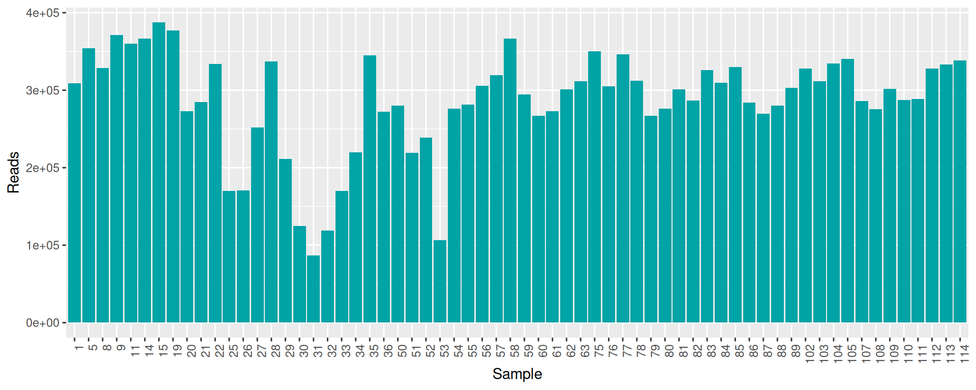

Code

raw_data %>% select(sample, num_seqs, sum_len, min_len, avg_len, max_len) %>% arrange(as.integer(sample)) %>% datatable()

Code

conda activate seqkit-2.0.0
cd /home/orue/work/PROJECTS/SCPWI/RAW_DATA/IC_Bre
seqkit stat --all -T -j 24 *.gz >> seqkit.txt
conda deactivate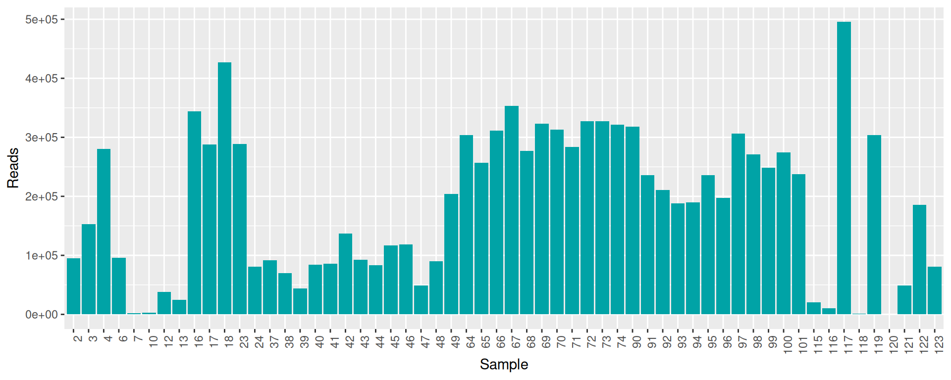

Code

raw_data %>% select(sample, num_seqs, sum_len, min_len, avg_len, max_len) %>% arrange(as.integer(sample)) %>% datatable(rownames = F)

Note

Some samples have a low number of reads. We keep them, but we could remove them at this step.

FastQC [3] is a program designed to spot potential problems in high througput sequencing datasets. It runs a set of analyses on one or more raw sequence files in fastq or bam format and produces a report which summarises the results. MultiQC [4] aggregates results from bioinformatics analyses across many samples into a single report.

Auzeville
Breteniere

Code

for i in RAW_DATA/IC_Auz/*.fastq.gz ; do echo "conda activate fastqc-0.11.9 && fastqc -t 8 $i -o QC/Auzeville/FASTQC && conda deactivate" >> fastqc_auz.sh ; done
qarray -cwd -V -N fastqc -pe thread 8 -o LOGS -e LOGS fastqc_auz.sh
qsub -cwd -V -N multiqc -o LOGS -e LOGS -b y "conda activate multiqc-1.11 && multiqc QC/Auzeville/FASTQC -o QC/Auzeville/MULTIQC && conda deactivate"

Here is the MultiQC report

Code

for i in RAW_DATA/IC_Bre/*.fastq.gz ; do echo "conda activate fastqc-0.11.9 && fastqc -t 8 $i -o QC/Breteniere/FASTQC && conda deactivate" >> fastqc_bre.sh ; done
qarray -cwd -V -N fastqc -pe thread 8 -o LOGS -e LOGS fastqc_bre.sh
qsub -cwd -V -N multiqc -o LOGS -e LOGS -b y "conda activate multiqc-1.11 && multiqc QC/Breteniere/FASTQC -o QC/Breteniere/MULTIQC && conda deactivate"

Here is the MultiQC report

Note

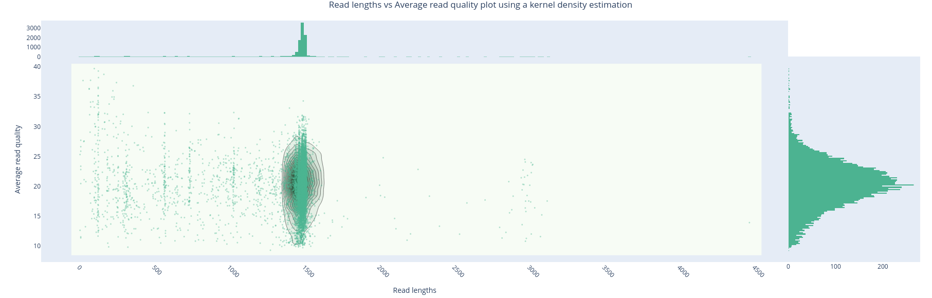
The metrics are expected for Nanopore reads. The quality is even quite good. The length distribution of reads shows short and very long reads that should not be present. We will remove them.

NanoPlot [5] is a plotting tool for long read sequencing data and alignments.

NanoStat [5] calculates various statistics from a long read sequencing dataset in fastq, bam or albacore sequencing summary format.

Auzeville
Breteniere

Code

for s in RAW_DATA/IC_Auz/*.fastq.gz ; do id=$(echo $(basename $s |cut -d '.' -f 1)) ; NanoPlot --outdir QC/Auzeville/NANOPLOT/ --prefix ${id} --tsv_stats --info_in_report --format png --fastq $s --threads 16 ; done

for s in RAW_DATA/IC_Auz/*.fastq.gz ; do id=$(echo $(basename $s |cut -d '.' -f 1)) ; NanoStat --fastq $s --outdir QC/Auzeville/NANOSTATS/ -n ${id} -t 16 ; done

Code

for s in RAW_DATA/IC_Bre/*.fastq.gz ; do id=$(echo $(basename $s |cut -d '.' -f 1)) ; NanoPlot --outdir QC/Breteniere/NANOPLOT/ --prefix ${id} --tsv_stats --info_in_report --format png --fastq $s --threads 16 ; done

for s in RAW_DATA/IC_Bre/*.fastq.gz ; do id=$(echo $(basename $s |cut -d '.' -f 1)) ; NanoStat --fastq $s --outdir QC/Breteniere/NANOSTATS/ -n ${id} -t 16 ; done

Note

Nanoplot and Nanostats give other quality metrics that I don’t show here because nothing abnormal was detected.

Cleaning

Chopper [5], intended for long read sequencing such as PacBio or ONT, filters and trims a fastq file.

Note

Filters used:

min GC: 0.3
max GC: 0.7
min length: 800
max length: 2000

Auzeville
Breteniere

Code

conda activate chopper-0.9.0
for s in RAW_DATA/IC_Auz/*.fastq.gz ; do id=$(echo $(basename $s |cut -d '.' -f 1)) ; gunzip -c $s | chopper -t 16 -q 10 --mingc 0.3 --maxgc 0.7 --minlength 800 --maxlength 2000 | gzip > CLEANING/Auzeville/${id}.fastq.gz ; done

Code

conda activate seqkit-2.0.0
cd /home/orue/work/PROJECTS/SCPWI/CLEANING/Auzeville
seqkit stat --all -T -j 24 *.gz >> seqkit.txt
conda deactivate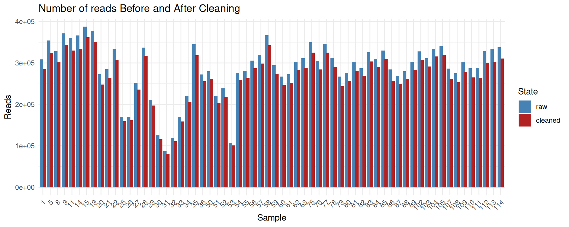

Code

raw_data <- read.csv2("data/seqkit_Auz.txt", stringsAsFactors = F, sep="", strip.white=T, dec=".") %>% as_tibble() %>% mutate(sample = basename(gsub('.fastq.gz$', '', file))) %>% distinct(sample, .keep_all = TRUE) %>% select(-file) %>% mutate(sum_len = as.numeric(gsub(",", "", sum_len))) %>% arrange(as.integer(sample)) %>% mutate(state = "raw", sum_len = as.integer(sum_len)) %>% select(sum_len, sample, state)

cleaned_data <- read.csv2("data/seqkit_Auz_cleaned.txt", stringsAsFactors = F, sep="", strip.white=T, dec=".") %>% as_tibble() %>% mutate(sample = basename(gsub('.fastq.gz$', '', file))) %>% distinct(sample, .keep_all = TRUE) %>% select(-file) %>% mutate(num_seqs = as.numeric(gsub(",", "", num_seqs))) %>% arrange(as.integer(sample)) %>% mutate(state = "cleaned", sum_len = as.integer(sum_len)) %>% select(sum_len, sample, state)

combined_data <- bind_rows(raw_data, cleaned_data)

combined_data <- combined_data %>%
  mutate(state = factor(state, levels = c("raw", "cleaned")))

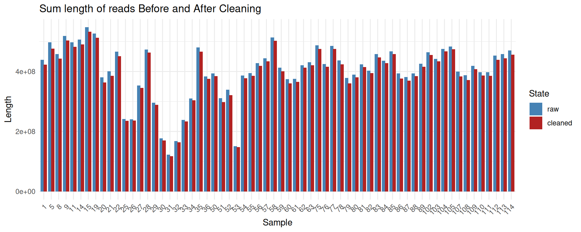
ggplot(combined_data, aes(x=reorder(sample, sort(as.numeric(sample))), y = sum_len, fill = state)) +
  geom_bar(stat = "identity", position = position_dodge(width = 0.8)) +
  scale_fill_manual(values = c("raw" = "steelblue", "cleaned" = "firebrick")) +
  labs(
    x = "Sample",
    y = "Length",
    fill = "State",
    title = "Sum length of reads Before and After Cleaning"
  ) +
  theme_minimal() +
  theme(
    axis.text.x = element_text(angle = 45, hjust = 1)
  )

Code

conda activate chopper-0.9.0
for s in RAW_DATA/IC_Bre/*.fastq.gz ; do id=$(echo $(basename $s |cut -d '.' -f 1)) ; gunzip -c $s | chopper -t 16 -q 10 --mingc 0.3 --maxgc 0.7 --minlength 800 --maxlength 2000 | gzip > CLEANING/Breteniere/${id}.fastq.gz ; done
conda deactivate

Code

conda activate seqkit-2.0.0
cd /home/orue/work/PROJECTS/SCPWI/CLEANING/Breteniere
seqkit stat --all -T -j 24 *.gz >> seqkit.txt
conda deactivate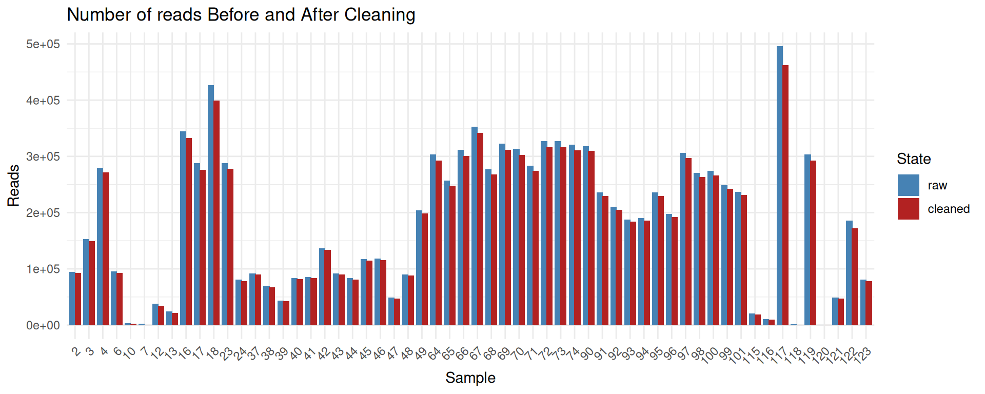

Code

raw_data <- read.csv2("data/seqkit_Bre.txt", stringsAsFactors = F, sep="", strip.white=T, dec=".") %>% as_tibble() %>% mutate(sample = basename(gsub('.fastq.gz$', '', file))) %>% distinct(sample, .keep_all = TRUE) %>% select(-file) %>% mutate(sum_len = as.numeric(gsub(",", "", sum_len))) %>% arrange(as.integer(sample)) %>% mutate(state = "raw", sum_len = as.integer(sum_len)) %>% select(sum_len, sample, state)

cleaned_data <- read.csv2("data/seqkit_Bre_cleaned.txt", stringsAsFactors = F, sep="", strip.white=T, dec=".") %>% as_tibble() %>% mutate(sample = basename(gsub('.fastq.gz$', '', file))) %>% distinct(sample, .keep_all = TRUE) %>% select(-file) %>% mutate(num_seqs = as.numeric(gsub(",", "", num_seqs))) %>% arrange(as.integer(sample)) %>% mutate(state = "cleaned", sum_len = as.integer(sum_len)) %>% select(sum_len, sample, state)

combined_data <- bind_rows(raw_data, cleaned_data)

combined_data <- combined_data %>%
  mutate(state = factor(state, levels = c("raw", "cleaned")))

ggplot(combined_data, aes(x=reorder(sample, sort(as.numeric(sample))), y = sum_len, fill = state)) +
  geom_bar(stat = "identity", position = position_dodge(width = 0.8)) +
  scale_fill_manual(values = c("raw" = "steelblue", "cleaned" = "firebrick")) +
  labs(
    x = "Sample",
    y = "Length",
    fill = "State",
    title = "Sum length of reads Before and After Cleaning"
  ) +
  theme_minimal() +
  theme(
    axis.text.x = element_text(angle = 45, hjust = 1)
  )

Note

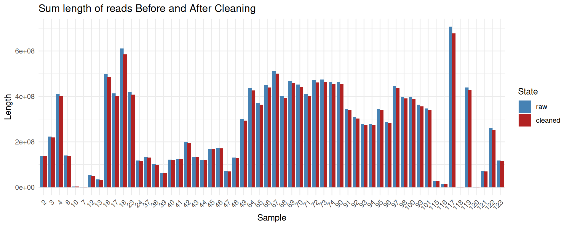
The cleaning process removes only a small fraction of reads and sequenced bases.

Code

cd /home/orue/work/PROJECTS/SCPWI

for s in RAW_DATA/IC_Bre/*.fastq.gz ; do id=$(echo $(basename $s |cut -d '.' -f 1)) ; NanoStat --fastq $s --outdir QC/Breteniere/NANOSTATS/ -n ${id} -t 16 ; done

Mapping

Minimap2 [6] is a versatile sequence alignment program that aligns DNA or mRNA sequences against a large reference database. Typical use cases include: (1) mapping PacBio or Oxford Nanopore genomic reads to the human genome; (2) finding overlaps between long reads with error rate up to ~15%; (3) splice-aware alignment of PacBio Iso-Seq or Nanopore cDNA or Direct RNA reads against a reference genome; (4) aligning Illumina single- or paired-end reads; (5) assembly-to-assembly alignment; (6) full-genome alignment between two closely related species with divergence below ~15%.

Code

cd /home/orue/work/PROJECTS/SCPWI/REFERENCES

conda activate minimap2-2.28
minimap2 SynCom_Ref16S_Auzeville.fasta -x ava-ont -d SynCom_Ref16S_Auzeville.mmi
minimap2 SynCom_Ref16S_Breteniere.fasta -x ava-ont -d SynCom_Ref16S_Breteniere.mmi

conda activate samtools-1.20 --stack

cd ../MAPPING
mkdir IC_Auz IC_Bre

## IC_Auz
date ; minimap2 -t 96 -ax map-ont -a REFERENCES/GTDB_16S_release220_202411/GTDB_16S_release220_202411.mmi CLEANING/Auzeville/81.fastq.gz |samtools view -bS - |samtools sort -m 16G -@ 96 - > MAPPING/Auzeville/81.bam ; date


for i in ../RAW_DATA/IC_Auz/*.gz ; do id=$(echo $(basename $i) |cut -d '.' -f 1) ; minimap2 -t 24 -ax map-ont -a ../REFERENCES/SynCom_Ref16S_Auzeville.mmi $i |samtools view -bS - |samtools sort - > IC_Auz/${id}.bam ; done
for i in IC_Auz/*.bam ; do samtools flagstat $i > $i.flagstat ; done
for i in IC_Auz/*.bam ; do samtools view $i |cut -f 3 |sort |uniq -c > $i.infos ; done

## IC_Bre
for i in ../RAW_DATA/IC_Bre/*.gz ; do id=$(echo $(basename $i) |cut -d '.' -f 1) ; minimap2 -t 24 -ax map-ont -a ../REFERENCES/SynCom_Ref16S_Breteniere.mmi $i |samtools view -bS - |samtools sort - > IC_Bre/${id}.bam ; done
for i in IC_Bre/*.bam ; do samtools view $i |cut -f 3 |sort |uniq -c > $i.infos ; done


for i in *.bam ; do samtools view -F 2048  $i  |cut -f 3 | sort |uniq -c | sort -k1,1nr |perl -lane 'print "$F[0]\t$F[1]"' > ${i}.counts ; done

conda deactivate


for i in CLEANING/Breteniere/*.gz ; do id=$(echo $(basename $i) |cut -d '.' -f 1) ; echo "conda activate minimap2-2.28 && conda activate samtools-1.20 --stack && minimap2 -t 64 -ax map-ont -a REFERENCES/GTDB_16S_release220_202411/GTDB_16S_release220_202411.mmi $i --secondary=no |samtools view -bS - |samtools sort -@ 64 - > MAPPING/Breteniere/${id}.bam" >> mapping_breteniere.sh ; done

Alignment files are filtered on FLAG to keep only the best hit of each read. Then, best hits counts are summed up.

Code

if(!file.exists("html/auzeville.rds")){
  file_path <- "data/IC_Auz"
  files <- list.files(file_path, pattern = "\\.bam\\.counts$", full.names = TRUE)
  
  data_list <- lapply(files, function(file) {
    data <- read.csv2(file, sep="\t", header = FALSE, col.names = c("reads", "GTDB_ID"))
    data$Sample <- gsub("\\.bam\\.counts$", "", basename(file))
    data <- data %>%
      mutate(GTDB_ID = ifelse(GTDB_ID == "*", "unknown", GTDB_ID)) %>% 
      mutate(Sample = str_trim(Sample)) %>% mutate(Sample = as.character(Sample))
    data
  })
  
  combined_data <- bind_rows(data_list)
  
  cdata <- combined_data %>% pivot_wider(names_from = Sample, values_from = reads, values_fill = 0)
  cdata2 <- left_join(cdata, refs, by="GTDB_ID") %>% separate(Taxonomy, ";(?=[\\S])", into = c("Kingdom","Phylum","Class","Order","Family","Genus","Species"), remove=FALSE) %>% rownames_to_column(var="OTUID") %>% mutate(OTUID = paste0("ASV_",OTUID))
  
  otumat = cdata2 %>% select(-OTUID, -GTDB_ID, -Taxonomy, -Kingdom, -Phylum, -Class, -Order, -Family, -Genus, -Species) %>% as.data.frame()
  rownames(otumat) <- cdata2$OTUID
  
  taxmat <- cdata2 %>% select(Kingdom, Phylum, Class, Order, Family, Genus, Species) %>% as.matrix()
  rownames(taxmat) <- rownames(otumat)
  
  OTU = otu_table(otumat, taxa_are_rows = TRUE)
  TAX = tax_table(taxmat)
  physeq = phyloseq(OTU, TAX)
  
  physeq
  
  sample_data(physeq) <- read.table("metadata.tsv", row.names = 1, header = TRUE, sep = "\t", stringsAsFactors = FALSE)
  
  
  clean_taxon_names <- function(taxon_column) {
    gsub("^[a-z]__| \\[id:.*\\]", "", taxon_column)
  }
  
  tax_table(physeq) <- apply(tax_table(physeq), 2, clean_taxon_names)
  
  
  saveRDS(physeq, "html/auzeville.rds")
}else{
  physeq <- readRDS("html/auzeville.rds")
}

Code

physeq

phyloseq-class experiment-level object
otu_table()   OTU Table:         [ 42016 taxa and 64 samples ]
sample_data() Sample Data:       [ 64 samples by 7 sample variables ]
tax_table()   Taxonomy Table:    [ 42016 taxa by 7 taxonomic ranks ]

Code

plot_composition(physeq, "Kingdom", "Bacteria", "Phylum", fill = "Phylum", numberOfTaxa = 20) +
  scale_fill_discrete() +
  facet_grid(~Compartment, scales = "free_x", space = "free_x")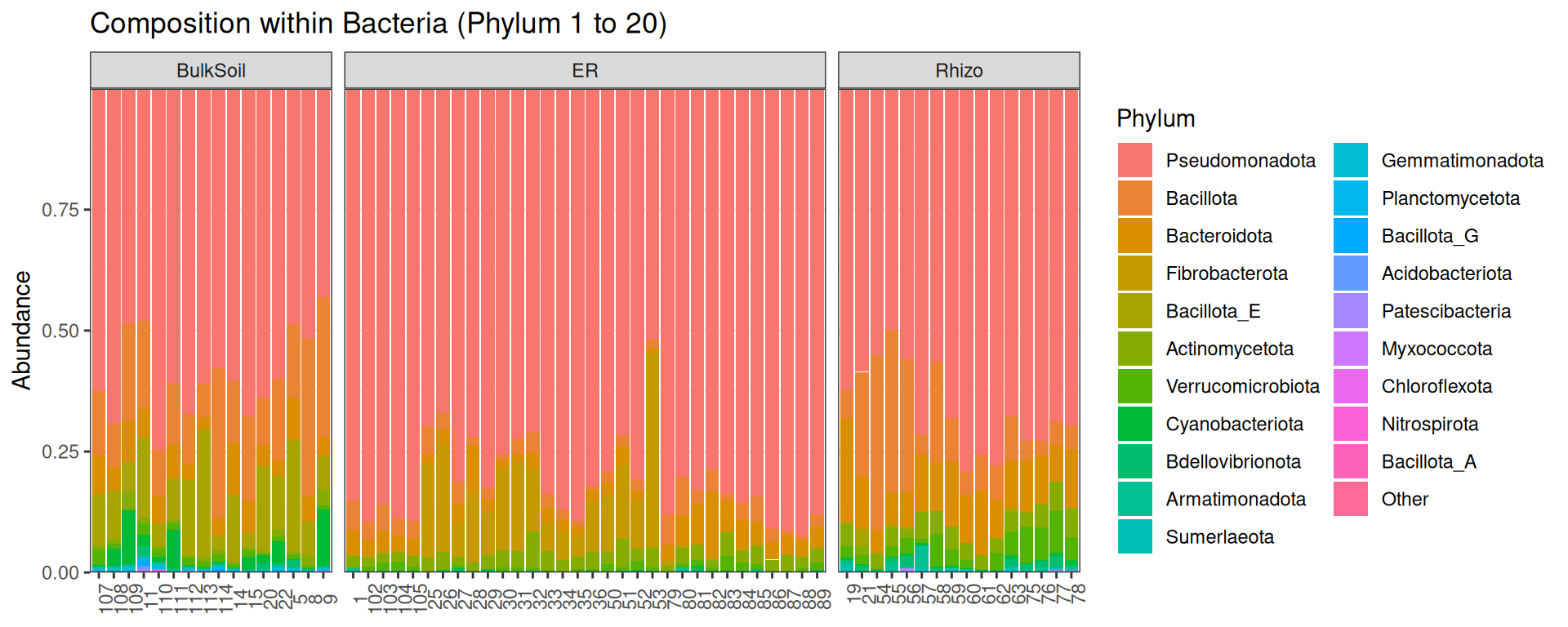

Code

p <- plot_composition(physeq, "Kingdom", "Bacteria", "Species", fill = "Species", numberOfTaxa = 20) +
  facet_grid(~Compartment, scales = "free_x", space = "free_x")
p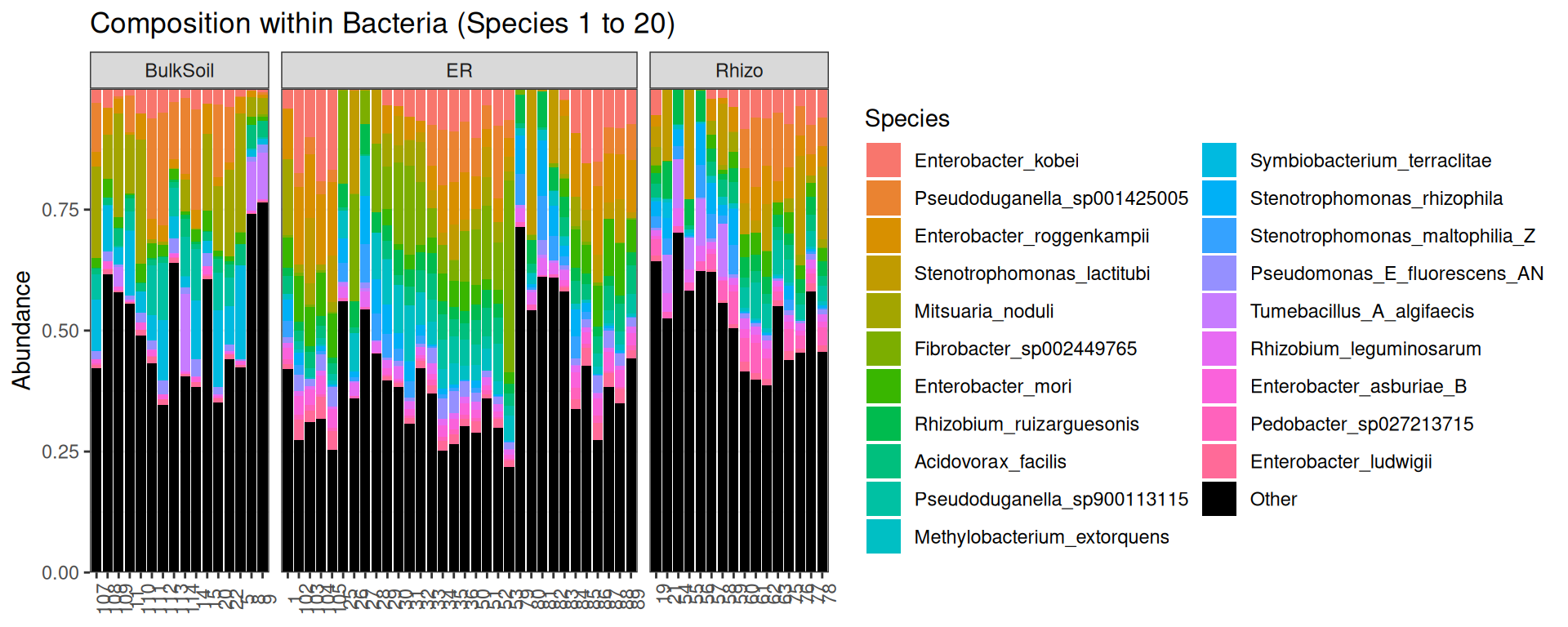

Code

if(!file.exists("html/breteniere.rds")){
  file_path <- "data/IC_Bre"
  files <- list.files(file_path, pattern = "\\.bam\\.counts$", full.names = TRUE)
  
  data_list <- lapply(files, function(file) {
    data <- read.csv2(file, sep="\t", header = FALSE, col.names = c("reads", "GTDB_ID"))
    data$Sample <- gsub("\\.bam\\.counts$", "", basename(file))
    data <- data %>%
      mutate(GTDB_ID = ifelse(GTDB_ID == "*", "unknown", GTDB_ID)) %>% 
      mutate(Sample = str_trim(Sample)) %>% mutate(Sample = as.character(Sample))
    data
  })
  
  combined_data <- bind_rows(data_list)
  
  cdata <- combined_data %>% pivot_wider(names_from = Sample, values_from = reads, values_fill = 0)
  cdata2 <- left_join(cdata, refs, by="GTDB_ID") %>% separate(Taxonomy, ";(?=[\\S])", into = c("Kingdom","Phylum","Class","Order","Family","Genus","Species"), remove=FALSE) %>% rownames_to_column(var="OTUID") %>% mutate(OTUID = paste0("ASV_",OTUID))
  
  otumat = cdata2 %>% select(-OTUID, -GTDB_ID, -Taxonomy, -Kingdom, -Phylum, -Class, -Order, -Family, -Genus, -Species) %>% as.data.frame()
  rownames(otumat) <- cdata2$OTUID
  
  taxmat <- cdata2 %>% select(Kingdom, Phylum, Class, Order, Family, Genus, Species) %>% as.matrix()
  rownames(taxmat) <- rownames(otumat)
  
  OTU = otu_table(otumat, taxa_are_rows = TRUE)
  TAX = tax_table(taxmat)
  physeq = phyloseq(OTU, TAX)
  
  physeq
  
  sample_data(physeq) <- read.table("metadata.tsv", row.names = 1, header = TRUE, sep = "\t", stringsAsFactors = FALSE)
  
  
  clean_taxon_names <- function(taxon_column) {
    gsub("^[a-z]__| \\[id:.*\\]", "", taxon_column)
  }
  
  tax_table(physeq) <- apply(tax_table(physeq), 2, clean_taxon_names)
  
  
  saveRDS(physeq, "html/breteniere.rds")
}else{
  physeq <- readRDS("html/breteniere.rds")
}

Code

physeq

phyloseq-class experiment-level object
otu_table()   OTU Table:         [ 28026 taxa and 58 samples ]
sample_data() Sample Data:       [ 58 samples by 7 sample variables ]
tax_table()   Taxonomy Table:    [ 28026 taxa by 7 taxonomic ranks ]

Code

plot_composition(physeq, "Kingdom", "Bacteria", "Phylum", fill = "Phylum", numberOfTaxa = 20) +
  scale_fill_discrete() +
  facet_grid(~Compartment, scales = "free_x", space = "free_x")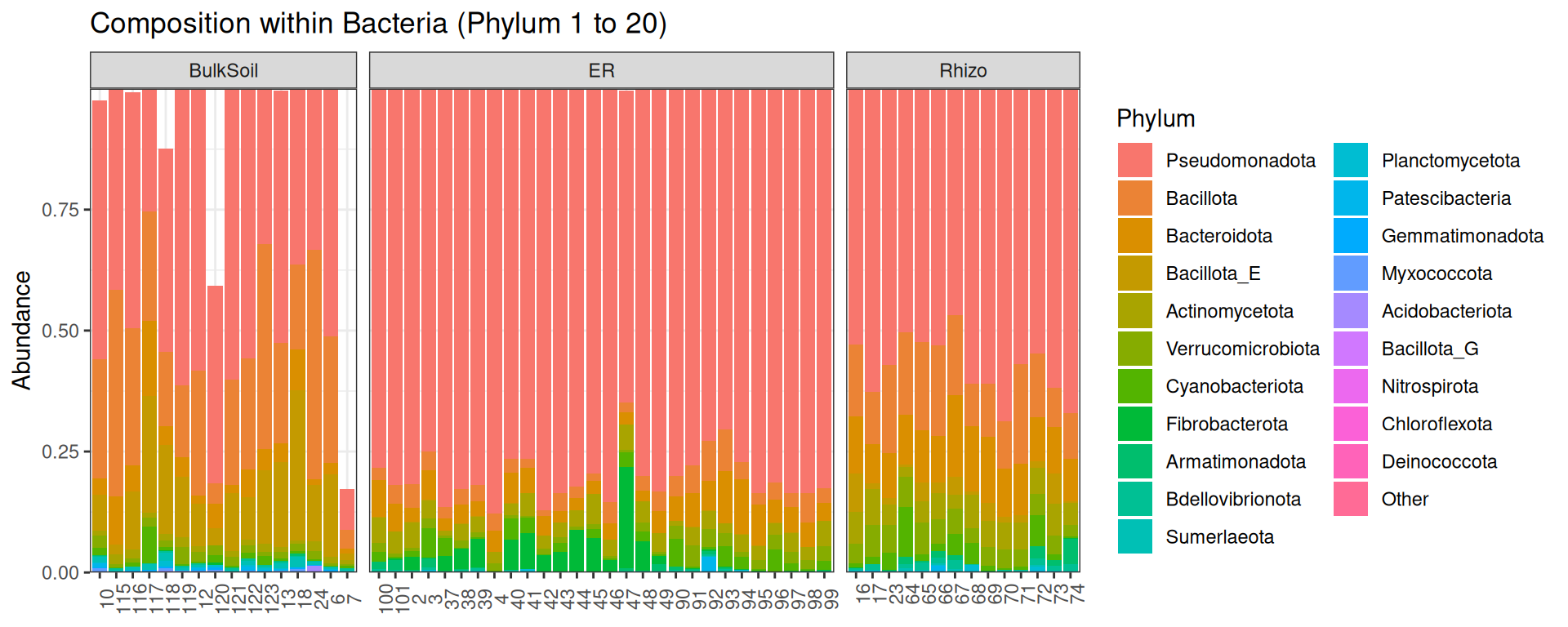

Code

p <- plot_composition(physeq, "Kingdom", "Bacteria", "Species", fill = "Species", numberOfTaxa = 20) +
  facet_grid(~Compartment, scales = "free_x", space = "free_x")
p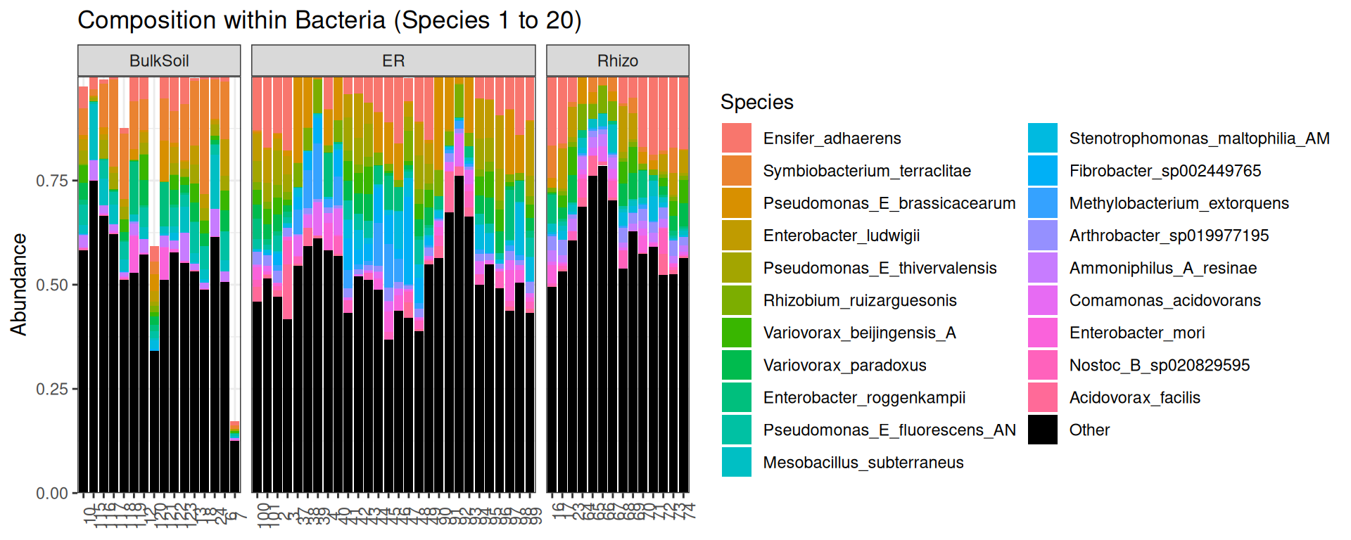

Downloads

The RDS files can be loaded in the Easy16S application

References

1. Altschul SF, Gish W, Miller W, Myers EW, Lipman DJ. Basic local alignment search tool. Journal of molecular biology. 1990;215:403–10.

2. Shen W, Le S, Li Y, Hu F. SeqKit: A cross-platform and ultrafast toolkit for FASTA/q file manipulation. PloS one. 2016;11:e0163962.

3. Andrews S. FastQC a quality control tool for high throughput sequence data. http://www.bioinformatics.babraham.ac.uk/projects/fastqc/. 2010. http://www.bioinformatics.babraham.ac.uk/projects/fastqc/.

4. Ewels P, Magnusson M, Lundin S, Käller M. MultiQC: Summarize analysis results for multiple tools and samples in a single report. Bioinformatics. 2016;32:3047–8.

5. De Coster W, Rademakers R. NanoPack2: population-scale evaluation of long-read sequencing data. Bioinformatics. 2023;39:btad311. doi:10.1093/bioinformatics/btad311.

6. Li H. Minimap2: Pairwise alignment for nucleotide sequences. Bioinformatics. 2018;34:3094–100.

Reuse

This document will not be accessible without prior agreement of the partners

A work by Migale Bioinformatics Facility
Université Paris-Saclay, INRAE, MaIAGE, 78350, Jouy-en-Josas, France
Université Paris-Saclay, INRAE, BioinfOmics, MIGALE bioinformatics facility, 78350, Jouy-en-Josas, France