RESILIENS-PILOTE

Note

This document is a report of the analyses performed. You will find all the code used to analyze these data. The version of the tools (maybe in code chunks) and their references are indicated, for questions of reproducibility.

Aim of the project

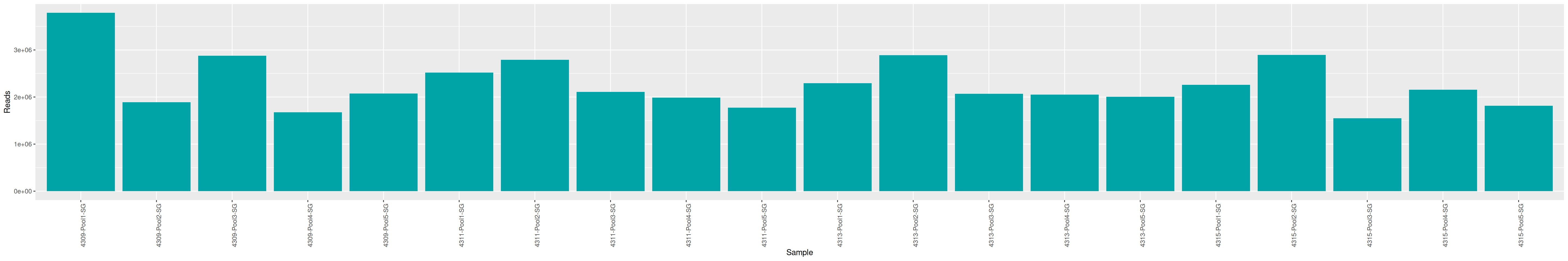
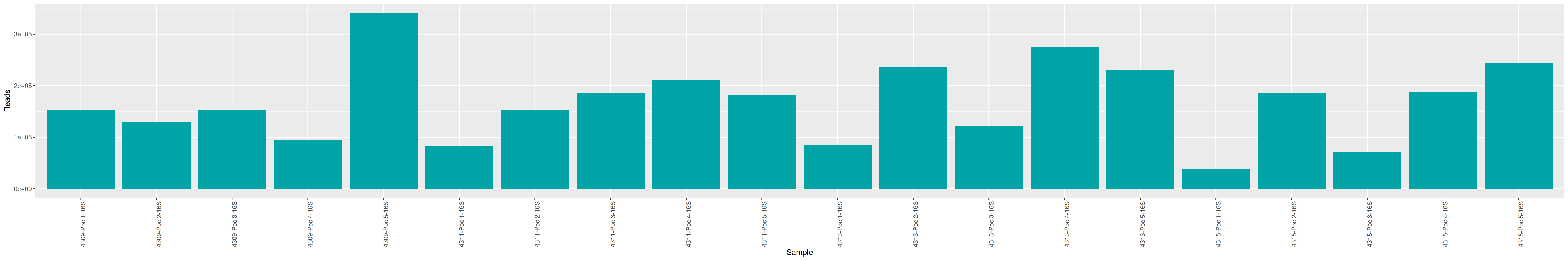
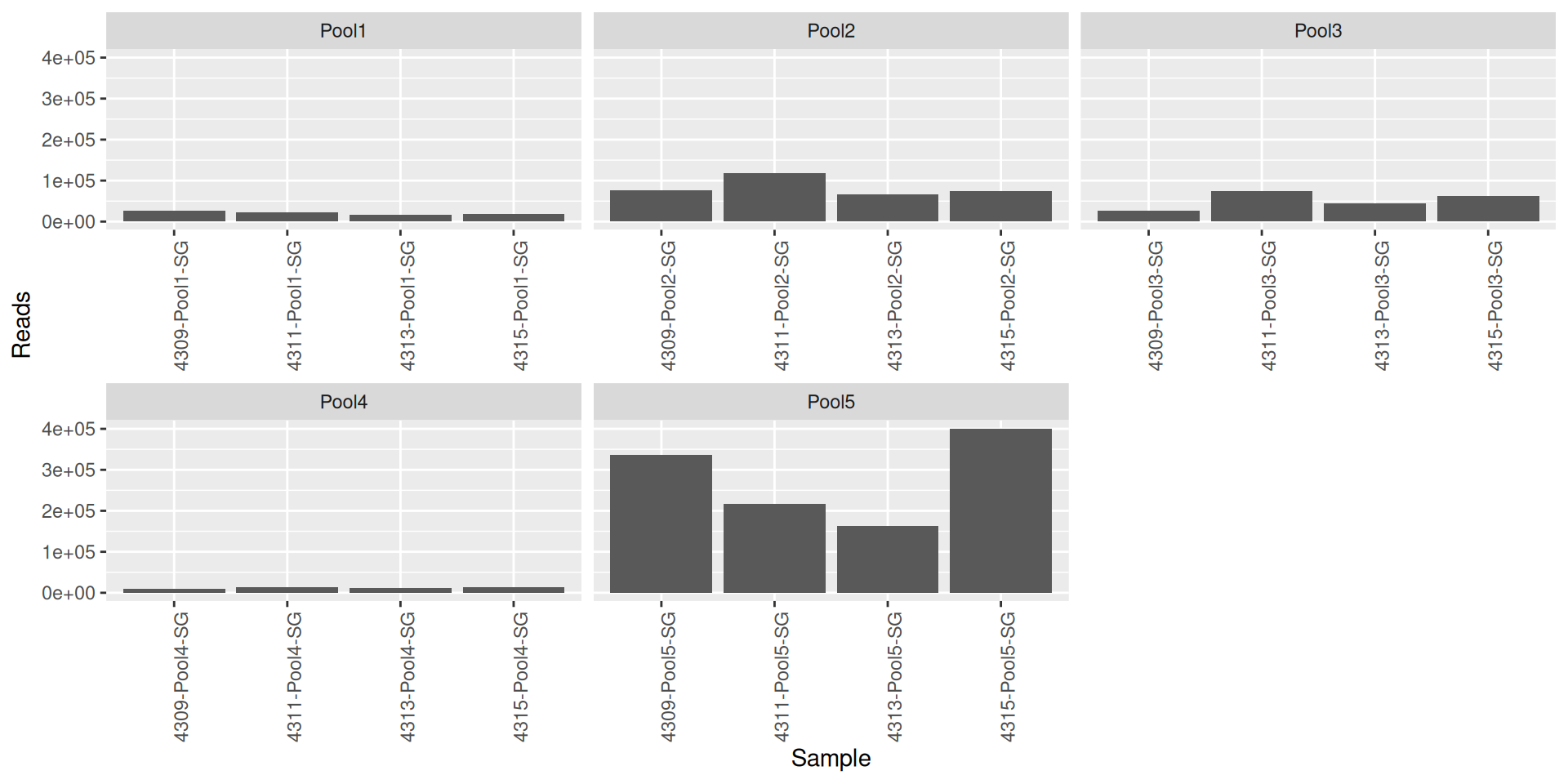
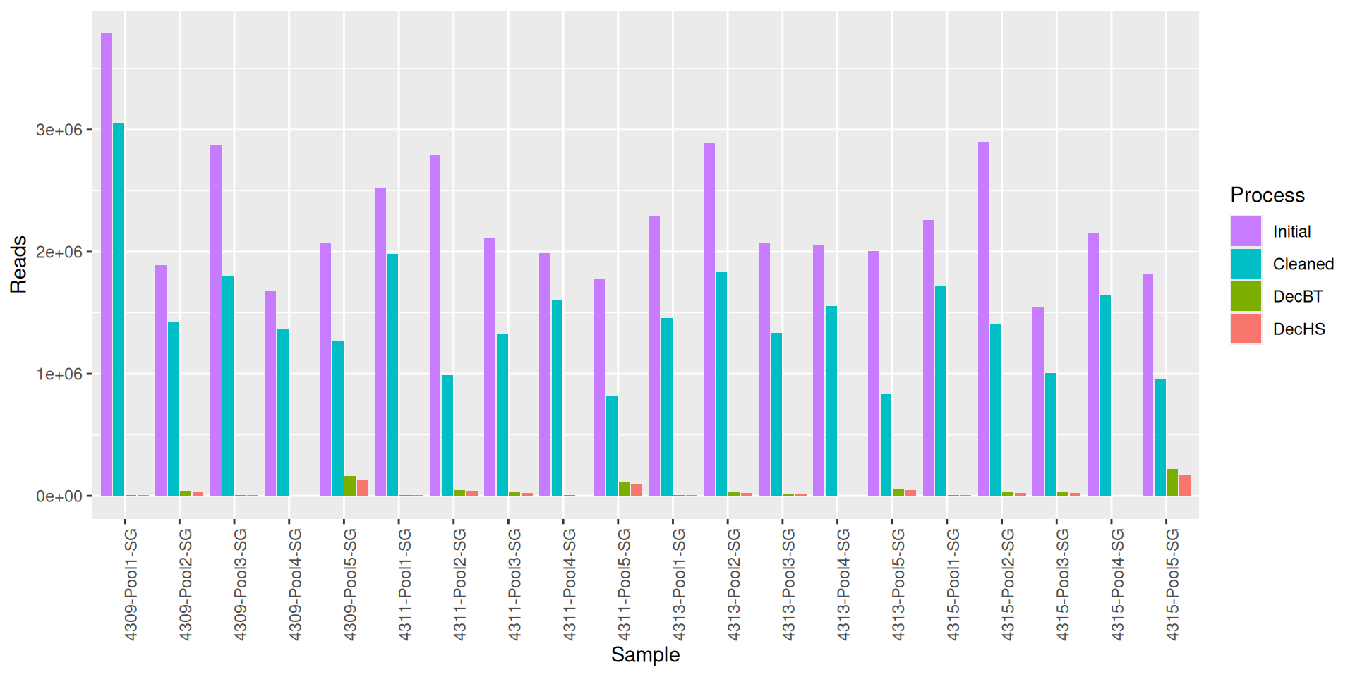
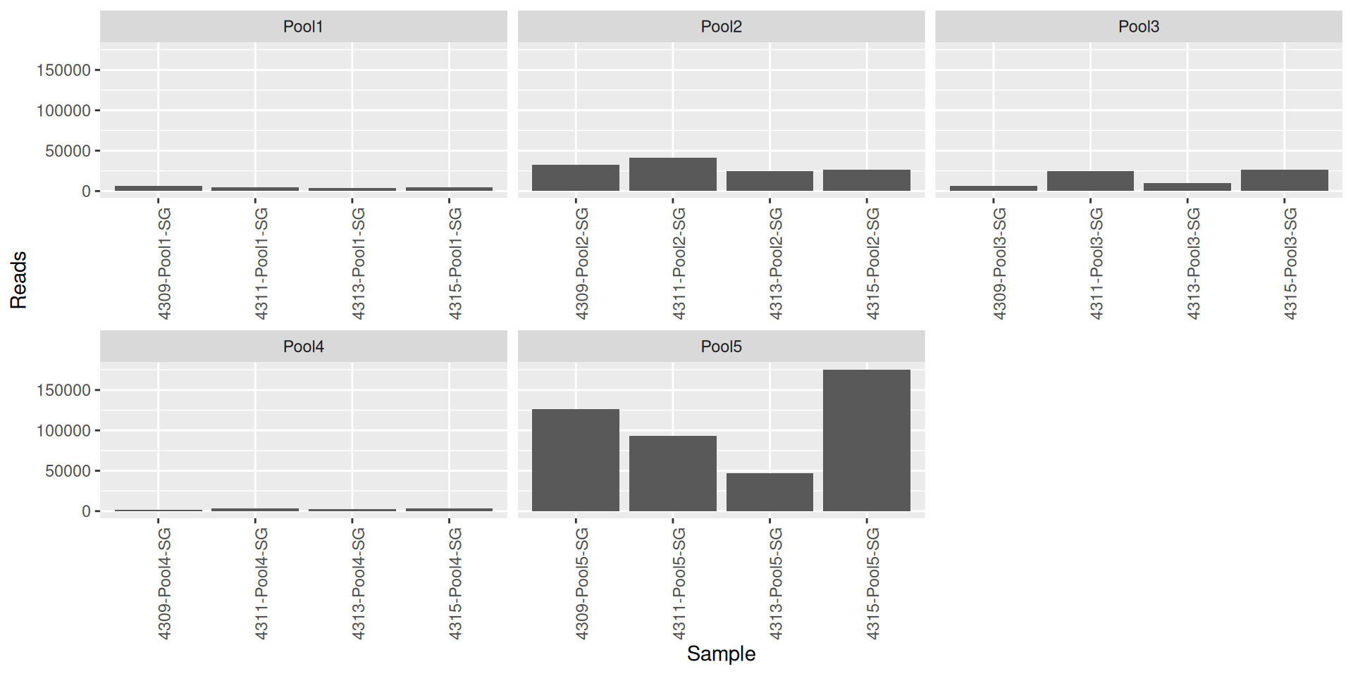
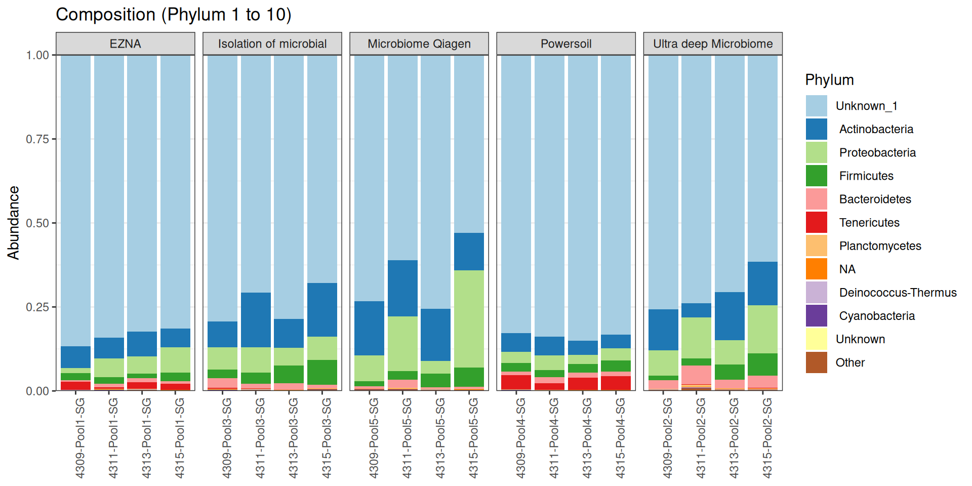
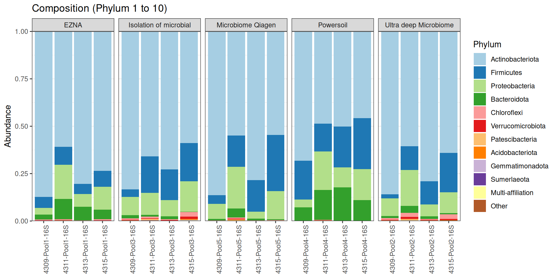
As part of the RESILIENS project, I sent 20 samples for shotgun sequencing to evaluate the efficiency of 5 different DNA extraction kits on 4 respiratory tract samples (4 different animals). The aim of this sequencing was to determine whether the different kits are able to deplete host DNA and thus increase the quantity of microbial reads. To begin with, 2 M reads PE 150bp x sample were requested. The same samples will also be sequenced by 16S sequencing in parallel to get an overview of the composition.

Partners

• Olivier Rué - Migale bioinformatics facility - BioInfomics - INRAE
• Valentin Loux - Migale bioinformatics facility - BioInfomics - INRAE
• Cédric Midoux - Migale bioinformatics facility - BioInfomics - INRAE
• Nuria Mach - UMR 1225 IHAP - INRAE

Deliverables

Deliverables agreed at the preliminary meeting (Table 1).

Table 1: Deliverables

	Definition	Status
1	HTML report	✔️

Data management

Important

All data is managed by the migale facility for the duration of the project. Once the project is over, the Migale facility does not keep your data. We will provide you with the raw data and associated metadata that will be deposited on public repositories before the results are used. We can guide you in the submission process. We will then decide which files to keep, knowing that this report will also be provided to you and that the analyses can be replayed if needed.

Raw data

The raw data were stored in the abaca server and on a dedicated space on the front server.

Bioinformatics

We first renamed FASTQ files.

cd /save_projet/resiliens/
mkdir -p PILOTE/16S PILOTE/SHOTGUN

cd PILOTE/SHOTGUN
mkdir RAW_DATA
cp /home/nmach/work/culturomics/shotgun/* .
for i in *_R1_*.fastq.gz ; do id=$(echo $i|cut -d '-' -f 2,3,4); mv $i RAW_DATA/${id}_R1.fastq.gz ; done
for i in *_R2_*.fastq.gz ; do id=$(echo $i|cut -d '-' -f 2,3,4); mv $i RAW_DATA/${id}_R2.fastq.gz ; done

cd ../16S
mkdir RAW_DATA
cp /home/nmach/work/culturomics/16S/*Pool* .
for i in *_R1_*.fastq.gz ; do id=$(echo $i|cut -d '-' -f 2,3,4); mv $i RAW_DATA/${id}_R1.fastq.gz ; done
for i in *_R2_*.fastq.gz ; do id=$(echo $i|cut -d '-' -f 2,3,4); mv $i RAW_DATA/${id}_R2.fastq.gz ; done
tar zcvf Resiliens-pilote.tar.gz *.fastq.gz

cd ../
scp -r * orue@abaca.maiage.inrae.fr:/backup/partage/migale/RESILIENS-PILOTE/

Quality control

Shotgun

seqkit [1] was used to get informations from FASTQ files.

# seqkit
cd /work_projet/resiliens/PILOTE/SHOTGUN
mkdir LOGS
qsub -cwd -V -o LOGS -e LOGS -N seqkit -pe thread 4 -R y -b y "conda activate seqkit-2.0.0 && seqkit stats /save_projet/resiliens/PILOTE/SHOTGUN/RAW_DATA/*.fastq.gz -j 4 
> raw_data.infos && conda deactivate"

We can plot and display the number of reads to see if enough reads are present and if samples are homogeneous.

FastQC [2] is a program designed to spot potential problems in high througput sequencing datasets. It runs a set of analyses on one or more raw sequence files in fastq or bam format and produces a report which summarises the results. MultiQC [3] aggregates results from bioinformatics analyses across many samples into a single report.

cd /work_projet/resiliens/PILOTE/SHOTGUN
mkdir FASTQC
for i in /save_projet/resiliens/PILOTE/SHOTGUN/RAW_DATA/*.fastq.gz ; do echo "conda activate fastqc-0.11.9 && fastqc $i -o FASTQC && conda deactivate" >> fastqc.sh ; done
qarray -cwd -V -N fastqc -o LOGS -e LOGS fastqc.sh
qsub -cwd -V -N multiqc -o LOGS -e LOGS -b y "conda activate multiqc-1.11 && multiqc FASTQC -o MULTIQC && conda deactivate"

The MultiQC report shows expected metrics for Illumina Hiseq sequencing data.

Note

The quality control shows a high N content in reads.

16S

seqkit [1] was used to get informations from FASTQ files.

# seqkit
cd /work_projet/resiliens/PILOTE/16S
mkdir LOGS
qsub -cwd -V -o LOGS -e LOGS -N seqkit -pe thread 4 -R y -b y "conda activate seqkit-2.0.0 && seqkit stats /save_projet/resiliens/PILOTE/16S/RAW_DATA/*.fastq.gz -j 4 
> raw_data.infos && conda deactivate"

We can plot and display the number of reads to see if enough reads are present and if samples are homogeneous.

FastQC [2] is a program designed to spot potential problems in high througput sequencing datasets. It runs a set of analyses on one or more raw sequence files in fastq or bam format and produces a report which summarises the results. MultiQC [3] aggregates results from bioinformatics analyses across many samples into a single report.

cd /work_projet/resiliens/PILOTE/16S/
mkdir FASTQC
for i in /save_projet/resiliens/PILOTE/16S/RAW_DATA/*.fastq.gz ; do echo "conda activate fastqc-0.11.9 && fastqc $i -o FASTQC && conda deactivate" >> fastqc.sh ; done
qarray -cwd -V -N fastqc -o LOGS -e LOGS fastqc.sh
qsub -cwd -V -N multiqc -o LOGS -e LOGS -b y "conda activate multiqc-1.11 && multiqc FASTQC -o MULTIQC && conda deactivate"

The MultiQC report shows expected metrics for Illumina Hiseq sequencing data.

Note

The quality control is good enough to go further. Nothing strange is detected at this stage.

Shotgun data analysis

Cleaning

fastp [4] is a tool designed to provide fast all-in-one preprocessing for FASTQ files. By default, this tool allows correction in overlapped regions (at least 30 bases between R1 and R2), removes reads with more than 5 ambiguous sequences, moves a sliding window from tail (3’) to front, drops the bases in the window if its mean quality < 30, stops otherwise. Reads shorter than 75 nucleotides are also removed.

cd /work_projet/resiliens/PILOTE/SHOTGUN
mkdir FASTP
for i in /save_projet/resiliens/PILOTE/SHOTGUN/RAW_DATA/*_R1.fastq.gz ; do id=$(echo $(basename $i | cut -d '_' -f 1)) ; echo "conda activate fastp-0.23.1 && fastp --in1 $i --in2 $(dirname $i)/${id}_R2.fastq.gz --out1 FASTP/${id}_R1.fastq.gz --out2 FASTP/${id}_R2.fastq.gz --verbose --length_required 50 --html FASTP/${id}_fastp.html --json FASTP/${id}_fastp.json --thread 4 && conda deactivate" >> fastp.sh ; done
qsub -cwd -V -N fastp -pe thread 4 -o LOGS/ -e LOGS/ fastp.sh

mkdir FASTQC
for i in /save_projet/resiliens/PILOTE/SHOTGUN/RAW_DATA/*.fastq.gz ; do echo "conda activate fastqc-0.11.9 && fastqc $i -o FASTQC && conda deactivate" >> fastqc.sh ; done
qarray -cwd -V -N fastqc -o LOGS -e LOGS fastqc.sh
qsub -cwd -V -N multiqc -o LOGS -e LOGS -b y "conda activate multiqc-1.11 && multiqc FASTQC -o MULTIQC && conda deactivate"

The MultiQC report after the cleaning process shows that a lot of reads with N have been removed, and the reads are now as good as possible.

data1 <- read.csv2("data/raw_data_shotgun.infos", stringsAsFactors = F, sep="", strip.white=T, dec=".") %>% as_tibble() %>% mutate(sample = basename(gsub('.{12}$', '', file))) %>% distinct(sample, .keep_all = TRUE) %>% select(-file) %>% mutate(num_seqs = as.numeric(gsub(",", "", num_seqs))) %>% dplyr::rename(Sample = sample) %>% mutate(Initial = num_seqs) %>% select(Sample, Initial)

data2 <- read.csv2("data/fastp.infos", stringsAsFactors = F, sep="", strip.white=T, dec=".") %>% as_tibble() %>% mutate(sample = basename(gsub('.{12}$', '', file))) %>% distinct(sample, .keep_all = TRUE) %>% select(-file) %>% mutate(num_seqs = as.numeric(gsub(",", "", num_seqs))) %>% dplyr::rename(Sample = sample) %>% mutate(Cleaned = num_seqs) %>% select(Sample, Cleaned)

data3 <- right_join(data1, data2) %>% gather(key="Process",value="Reads", -Sample)

p <- ggplot(data=data3, aes(x=Sample, y=Reads, fill=Process)) +
      xlab("Sample")  + ylab("Reads") +
      scale_y_continuous() +
     geom_bar(stat="identity", position=position_dodge2(reverse = TRUE)) +
  theme(axis.text.x = element_text(angle = 90, hjust = 1)) +
  scale_color_inrae() +
  guides(fill = guide_legend(reverse = TRUE)) 
p

Contamination

HoCoRT [5] stands for Host Contamination Removal Tool. Its purpose is to simplify and improve the process of host contamination removal from sequencing reads. It does not do any quality checking or low complexity region masking, just host contamination removal. HoCoRT wraps already existing aligners and classifiers such as Bowtie2 and Kraken2 to remove host contamination.

1. The sequencing data is mapped to the reference genome.
2. The sequences which map well are removed and the remaining sequences are written to output files.

Some of the pipelines combine multiple mappers/classifiers in an attempt to improve the results.

The reference bovine and human genomes, ARS-UCD2.0 and GRCh38.p14, were downloaded from the NCBI website and used with HOCORT. Bwa-mem2 and Bowtie2 was tested for mapping strategy.

conda activate hocort-1.2.2

cd /work_projet/resiliens/
hocort index bwamem2 -i /save_projet/resiliens/GCF_002263795.3_ARS-UCD2.0_genomic.fna -o ./bwamem
hocort index kraken2 -i /save_projet/resiliens/GCF_002263795.3_ARS-UCD2.0_genomic.fna -o ./k2 -t 16
hocort index bowtie2 -i /save_projet/resiliens/GCF_002263795.3_ARS-UCD2.0_genomic.fna -o ./bt2

hocort index bowtie2 -i /save_projet/resiliens/GCF_000001405.40_GRCh38.p14_genomic.fna -o ./human_bt2
hocort index bwamem2 -i /save_projet/resiliens/GCF_000001405.40_GRCh38.p14_genomic.fna -o ./human_bwamem2

mkdir HOCORT/BT/
mkdir HOCORT/BT/BWAMEM2
mkdir HOCORT/BT/BOWTIE2

for i in /work_projet/resiliens/PILOTE/SHOTGUN/FASTP/*_R1.fastq.gz ; do id=$(echo $(basename $i |cut -d '_' -f 1)) ;  hocort map bwamem2 -x bwamem  -i $i $(dirname $i)/${id}_R2.fastq.gz -o HOCORT/BT/BWAMEM2/${id}_R1.fastq.gz HOCORT/BT/BWAMEM2/${id}_R2.fastq.gz -t 16 --filter true ; done
for i in /work_projet/resiliens/PILOTE/SHOTGUN/FASTP/*_R1.fastq.gz ; do id=$(echo $(basename $i |cut -d '_' -f 1)) ;  hocort map bowtie2 -x bt2  -i $i $(dirname $i)/${id}_R2.fastq.gz -o HOCORT/BT/BOWTIE2/${id}_R1.fastq.gz HOCORT/BT/BOWTIE2/${id}_R2.fastq.gz -t 16 --filter true ; done


mkdir HOCORT/HS/
mkdir HOCORT/HS/BWAMEM2
mkdir HOCORT/HS/BOWTIE2

for i in HOCORT/BT/BWAMEM2/*_R1.fastq.gz ; do id=$(echo $(basename $i |cut -d '_' -f 1)) ;  hocort map bwamem2 -x human_bwamem2  -i $i $(dirname $i)/${id}_R2.fastq.gz -o HOCORT/HS/BWAMEM2/${id}_R1.fastq.gz HOCORT/HS/BWAMEM2/${id}_R2.fastq.gz -t 16 --filter true ; done
for i in HOCORT/BT/BOWTIE2/*_R1.fastq.gz ; do id=$(echo $(basename $i |cut -d '_' -f 1)) ;  hocort map bowtie2 -x human_bt2  -i $i $(dirname $i)/${id}_R2.fastq.gz -o HOCORT/HS/BOWTIE2/${id}_R1.fastq.gz HOCORT/HS/BOWTIE2/${id}_R2.fastq.gz -t 16 --filter true ; done


cd HOCORT/BWAMEM2
conda activate seqkit-2.0.0 && seqkit stats *.fastq.gz -j 4 > hocort_data.infos && conda deactivate

Bowtie2

data1 <- read.csv2("data/raw_data_shotgun.infos", stringsAsFactors = F, sep="", strip.white=T, dec=".") %>% as_tibble() %>% mutate(sample = basename(gsub('.{12}$', '', file))) %>% distinct(sample, .keep_all = TRUE) %>% select(-file) %>% mutate(num_seqs = as.numeric(gsub(",", "", num_seqs))) %>% dplyr::rename(Sample = sample) %>% mutate(Initial = num_seqs) %>% select(Sample, Initial)

data2 <- read.csv2("data/fastp.infos", stringsAsFactors = F, sep="", strip.white=T, dec=".") %>% as_tibble() %>% mutate(sample = basename(gsub('.{12}$', '', file))) %>% distinct(sample, .keep_all = TRUE) %>% select(-file) %>% mutate(num_seqs = as.numeric(gsub(",", "", num_seqs))) %>% dplyr::rename(Sample = sample) %>% mutate(Cleaned = num_seqs) %>% select(Sample, Cleaned)

data3 <- read.csv2("data/hcort_bt_bt2.infos", stringsAsFactors = F, sep="", strip.white=T, dec=".") %>% as_tibble() %>% mutate(sample = basename(gsub('.{12}$', '', file))) %>% distinct(sample, .keep_all = TRUE) %>% select(-file) %>% mutate(num_seqs = as.numeric(gsub(",", "", num_seqs))) %>% dplyr::rename(Sample = sample) %>% mutate(DecBT = num_seqs) %>% select(Sample, DecBT)

data4 <- read.csv2("data/hcort_hs_bt2.infos", stringsAsFactors = F, sep="", strip.white=T, dec=".") %>% as_tibble() %>% mutate(sample = basename(gsub('.{12}$', '', file))) %>% distinct(sample, .keep_all = TRUE) %>% select(-file) %>% mutate(num_seqs = as.numeric(gsub(",", "", num_seqs))) %>% dplyr::rename(Sample = sample) %>% mutate(DecHS = num_seqs) %>% select(Sample, DecHS)

data5 <- right_join(data1, data2) %>% right_join(., data3, by="Sample") %>% right_join(., data4, by="Sample")

data5 %>% mutate(Remaining=formatC(num(DecHS/Initial*100, label = "%", scale = 100), digits=3)) %>% datatable()

data_final <- data5 %>% gather(key="Process",value="Reads", -Sample)
p <- ggplot(data=data_final, aes(x=Sample, y=Reads, fill=reorder(Process, Reads))) +
      xlab("Sample")  + ylab("Reads") +
      scale_y_continuous() +
     geom_bar(stat="identity", position=position_dodge2(reverse = TRUE)) +
  theme(axis.text.x = element_text(angle = 90, hjust = 1)) +
  scale_color_inrae() +
  guides(fill = guide_legend(reverse = TRUE)) + scale_fill_discrete(name = "Process")
p

data_final2 <- data_final %>% filter(Process == "DecHS") %>% select(Sample, Reads) %>% mutate(Pool=str_extract(Sample,"Pool\\d+"))
p <- ggplot(data=data_final2) +
      xlab("Sample")  + ylab("Reads") +
  geom_col(aes(x=Sample,y=Reads)) +
  facet_wrap(~Pool, scales= "free_x") +
  theme(axis.text.x = element_text(angle = 90, hjust = 1))
p

Bwa-mem2

data1 <- read.csv2("data/raw_data_shotgun.infos", stringsAsFactors = F, sep="", strip.white=T, dec=".") %>% as_tibble() %>% mutate(sample = basename(gsub('.{12}$', '', file))) %>% distinct(sample, .keep_all = TRUE) %>% select(-file) %>% mutate(num_seqs = as.numeric(gsub(",", "", num_seqs))) %>% dplyr::rename(Sample = sample) %>% mutate(Initial = num_seqs) %>% select(Sample, Initial)

data2 <- read.csv2("data/fastp.infos", stringsAsFactors = F, sep="", strip.white=T, dec=".") %>% as_tibble() %>% mutate(sample = basename(gsub('.{12}$', '', file))) %>% distinct(sample, .keep_all = TRUE) %>% select(-file) %>% mutate(num_seqs = as.numeric(gsub(",", "", num_seqs))) %>% dplyr::rename(Sample = sample) %>% mutate(Cleaned = num_seqs) %>% select(Sample, Cleaned)

data3 <- read.csv2("data/hcort_bt_bwamem2.infos", stringsAsFactors = F, sep="", strip.white=T, dec=".") %>% as_tibble() %>% mutate(sample = basename(gsub('.{12}$', '', file))) %>% distinct(sample, .keep_all = TRUE) %>% select(-file) %>% mutate(num_seqs = as.numeric(gsub(",", "", num_seqs))) %>% dplyr::rename(Sample = sample) %>% mutate(DecBT = num_seqs) %>% select(Sample, DecBT)

data4 <- read.csv2("data/hcort_hs_bwamem2.infos", stringsAsFactors = F, sep="", strip.white=T, dec=".") %>% as_tibble() %>% mutate(sample = basename(gsub('.{12}$', '', file))) %>% distinct(sample, .keep_all = TRUE) %>% select(-file) %>% mutate(num_seqs = as.numeric(gsub(",", "", num_seqs))) %>% dplyr::rename(Sample = sample) %>% mutate(DecHS = num_seqs) %>% select(Sample, DecHS)

data5 <- right_join(data1, data2) %>% right_join(., data3, by="Sample") %>% right_join(., data4, by="Sample")

data5 %>% mutate(Remaining=formatC(num(DecHS/Initial*100, label = "%", scale = 100), digits=3)) %>% datatable()

data_final <- data5 %>% gather(key="Process",value="Reads", -Sample)

p <- ggplot(data=data_final, aes(x=Sample, y=Reads, fill=reorder(Process, Reads))) +
      xlab("Sample")  + ylab("Reads") +
      scale_y_continuous() +
     geom_bar(stat="identity", position=position_dodge2(reverse = TRUE)) +
  theme(axis.text.x = element_text(angle = 90, hjust = 1)) +
  scale_color_inrae() +
  guides(fill = guide_legend(reverse = TRUE)) + scale_fill_discrete(name = "Process")
p

data_final2 <- data_final %>% filter(Process == "DecHS") %>% select(Sample, Reads) %>% mutate(Pool=str_extract(Sample,"Pool\\d+"))
p <- ggplot(data=data_final2) +
      xlab("Sample")  + ylab("Reads") +
  geom_col(aes(x=Sample,y=Reads)) +
  facet_wrap(~Pool, scales= "free_x") +
  theme(axis.text.x = element_text(angle = 90, hjust = 1)) +
  scale_color_inrae() 
p

Note

The decontamination process shows a high proportion of Bos Taurus reads, and a very small proportion of human reads. The Pool5 (=Microbiome Qiagen extraction kit) samples demonstrate the lowest contamination rate.

Taxonomic affiliation of decontaminated reads

Kaiju [6] is a program for fast and sensitive taxonomic classification of high-throughput sequencing reads from metagenomic whole genome sequencing or metatranscriptomics experiments.

Each sequencing read is assigned to a taxon in the NCBI taxonomy by comparing it to a reference protein database containing microbial and viral protein sequences. By using protein-level classification, Kaiju achieves a higher sensitivity compared with methods based on nucleotide comparison.

The refseq databank was used (and one test with the progenomes databank).

Reads without affiliation (unknown phylum) were discarded in the second plot.

conda activate kaiju-1.9.2
for i in HOCORT/HS/BOWTIE2/*_R1.fastq.gz ; do id=$(echo $(basename $i |cut -d '_' -f 1)) ; kaiju -t /db/outils/kaiju-2021-03/refseq/nodes.dmp -f /db/outils/kaiju-2021-03/refseq/kaiju_db_refseq.fmi -i $i -j $(dirname $i)/${id}_R2.fastq.gz -o KAIJU_CLEANED_DECONTA/BOWTIE2/${id} -z 16 ; done
for i in KAIJU_CLEANED_DECONTA/BOWTIE2/* ; do kaiju-addTaxonNames -i $i -t /db/outils/kaiju-2021-03/refseq/nodes.dmp -n /db/outils/kaiju-2021-03/refseq/names.dmp -r superkingdom,phylum,order,class,family,genus,species  > $i.names ; done
python kaiju2phyloseq.py --indir KAIJU_CLEANED_DECONTA/BOWTIE2/ --names /db/outils/kaiju-2021-03/refseq/names.dmp --nodes /db/outils/kaiju-2021-03/refseq/nodes.dmp --output KAIJU_CLEANED_DECONTA/BOWTIE2/kaiju_refseq

for i in HOCORT/HS/BWAMEM2/*_R1.fastq.gz ; do id=$(echo $(basename $i |cut -d '_' -f 1)) ; kaiju -t /db/outils/kaiju-2021-03/refseq/nodes.dmp -f /db/outils/kaiju-2021-03/refseq/kaiju_db_refseq.fmi -i $i -j $(dirname $i)/${id}_R2.fastq.gz -o KAIJU_CLEANED_DECONTA/BWAMEM2/${id} -z 16 ; done
for i in KAIJU_CLEANED_DECONTA/BWAMEM2/* ; do kaiju-addTaxonNames -i $i -t /db/outils/kaiju-2021-03/refseq/nodes.dmp -n /db/outils/kaiju-2021-03/refseq/names.dmp -r superkingdom,phylum,order,class,family,genus,species  > $i.names ; done
python kaiju2phyloseq.py --indir KAIJU_CLEANED_DECONTA/BWAMEM2/ --names /db/outils/kaiju-2021-03/refseq/names.dmp --nodes /db/outils/kaiju-2021-03/refseq/nodes.dmp --output KAIJU_CLEANED_DECONTA/BWAMEM2/kaiju_refseq

## Progenomes

for i in HOCORT/HS/BWAMEM2/*_R1.fastq.gz ; do id=$(echo $(basename $i |cut -d '_' -f 1)) ; kaiju -t /db/outils/kaiju-2021-03/progenomes/nodes.dmp -f /db/outils/kaiju-2021-03/progenomes/kaiju_db_progenomes.fmi -i $i -j $(dirname $i)/${id}_R2.fastq.gz -o KAIJU_CLEANED_DECONTA/BWAMEM2/${id}.progenomes -z 16 ; done
for i in KAIJU_CLEANED_DECONTA/BWAMEM2/*.progenomes ; do kaiju-addTaxonNames -i $i -t /db/outils/kaiju-2021-03/progenomes/nodes.dmp -n /db/outils/kaiju-2021-03/progenomes/names.dmp -r superkingdom,phylum,order,class,family,genus,species  > $i.names ; done
mkdir KAIJU_CLEANED_DECONTA/BWAMEM2/PROGENOMES/
mv KAIJU_CLEANED_DECONTA/BWAMEM2/*progenomes* PROGENOMES/
python kaiju2phyloseq.py --indir KAIJU_CLEANED_DECONTA/BWAMEM2/PROGENOMES/ --names /db/outils/kaiju-2021-03/progenomes/names.dmp --nodes /db/outils/kaiju-2021-03/progenomes/nodes.dmp --output KAIJU_CLEANED_DECONTA/BWAMEM2/PROGENOMES/kaiju_progenomes

Bowtie2

otutab <- read.csv("data/kaiju_refseq_bt2.otu.tab", sep = "\t", row.names = 1, header = TRUE, stringsAsFactors = FALSE, check.names = F)
colnames(otutab) <- str_replace(colnames(otutab),".names","")
OTU = otu_table(otutab, taxa_are_rows = TRUE)

taxtab <- read.csv("data/kaiju_refseq_bt2.tax.tab", sep = "\t", row.names = 1, header = TRUE)
taxmat = as.matrix(taxtab)
TAX = tax_table(taxmat)

metadata <- read.table("data/metadata_shotgun.txt", row.names = 1, header = TRUE, sep = "\t", stringsAsFactors = FALSE)

physeq = phyloseq(OTU, TAX)
sample_data(physeq) <- metadata
physeq

phyloseq-class experiment-level object
otu_table()   OTU Table:         [ 5440 taxa and 20 samples ]
sample_data() Sample Data:       [ 20 samples by 4 sample variables ]
tax_table()   Taxonomy Table:    [ 5440 taxa by 7 taxonomic ranks ]

badTaxa = c("OTU00001")
allTaxa = taxa_names(physeq)
allTaxa <- allTaxa[!(allTaxa %in% badTaxa)]
physeq_known = prune_taxa(allTaxa, physeq)

plot_composition(physeq, taxaRank1 = "Bacteria", taxaSet1 = NULL, taxaRank2 = "Phylum", numberOfTaxa = 10) + 
  scale_fill_brewer(palette = "Paired") +
  facet_grid(~Extraction_kit, scales = "free_x", space = "free_x")

Problematic taxa
             taxa  Domain  Phylum rank
OTU00001 OTU00001 Unknown Unknown    1

plot_composition(physeq_known, taxaRank1 = "Bacteria", taxaSet1 = NULL, taxaRank2 = "Phylum", numberOfTaxa = 10) + 
  scale_fill_brewer(palette = "Paired") +
  facet_grid(~Extraction_kit, scales = "free_x", space = "free_x")

saveRDS(physeq,"html/resisiliens-pilote.shotgun.physeq.bt2.rds")

Bwa-mem2

otutab <- read.csv("data/kaiju_refseq_bwamem2.otu.tab", sep = "\t", row.names = 1, header = TRUE, stringsAsFactors = FALSE, check.names = F)
colnames(otutab) <- str_replace(colnames(otutab),".names","")
OTU = otu_table(otutab, taxa_are_rows = TRUE)

taxtab <- read.csv("data/kaiju_refseq_bwamem2.tax.tab", sep = "\t", row.names = 1, header = TRUE)
taxmat = as.matrix(taxtab)
TAX = tax_table(taxmat)

metadata <- read.table("data/metadata_shotgun.txt", row.names = 1, header = TRUE, sep = "\t", stringsAsFactors = FALSE)

physeq = phyloseq(OTU, TAX)
sample_data(physeq) <- metadata
physeq 

phyloseq-class experiment-level object
otu_table()   OTU Table:         [ 4890 taxa and 20 samples ]
sample_data() Sample Data:       [ 20 samples by 4 sample variables ]
tax_table()   Taxonomy Table:    [ 4890 taxa by 7 taxonomic ranks ]

#plot_bar(physeq, fill="Phylum") + facet_wrap(~Extraction_kit, scales= "free_x", nrow=1)

badTaxa = c("OTU00001")
allTaxa = taxa_names(physeq)
allTaxa <- allTaxa[!(allTaxa %in% badTaxa)]
physeq_known = prune_taxa(allTaxa, physeq)

plot_composition(physeq, taxaRank1 = "Bacteria", taxaSet1 = NULL, taxaRank2 = "Phylum", numberOfTaxa = 10) + 
  scale_fill_brewer(palette = "Paired") +
  facet_grid(~Extraction_kit, scales = "free_x", space = "free_x")

Problematic taxa
             taxa  Domain  Phylum rank
OTU00001 OTU00001 Unknown Unknown    1

plot_composition(physeq_known, taxaRank1 = "Bacteria", taxaSet1 = NULL, taxaRank2 = "Phylum", numberOfTaxa = 10) + 
  scale_fill_brewer(palette = "Paired") +
  facet_grid(~Extraction_kit, scales = "free_x", space = "free_x")

saveRDS(physeq,"html/resisiliens-pilote.shotgun.physeq.bwamem2.rds")

Bwa-mem2 progenomes

otutab <- read.csv("data/kaiju_progenomes.otu.tab", sep = "\t", row.names = 1, header = TRUE, stringsAsFactors = FALSE, check.names = F, strip.white = T)
colnames(otutab) <- str_replace(colnames(otutab),".progenomes.names","")
OTU = otu_table(otutab, taxa_are_rows = TRUE)

taxtab <- read.csv("data/kaiju_progenomes.tax.tab", sep = "\t", row.names = 1, header = TRUE, strip.white = T)
taxmat = as.matrix(taxtab)
TAX = tax_table(taxmat)

metadata <- read.table("data/metadata_shotgun.txt", row.names = 1, header = TRUE, sep = "\t", stringsAsFactors = FALSE)

physeq = phyloseq(OTU, TAX)
sample_data(physeq) <- metadata
physeq 

phyloseq-class experiment-level object
otu_table()   OTU Table:         [ 8210 taxa and 20 samples ]
sample_data() Sample Data:       [ 20 samples by 4 sample variables ]
tax_table()   Taxonomy Table:    [ 8210 taxa by 7 taxonomic ranks ]

#plot_bar(physeq, fill="Phylum") + facet_wrap(~Extraction_kit, scales= "free_x", nrow=1)

badTaxa = c("OTU00003", "OTU00078")
allTaxa = taxa_names(physeq)
allTaxa <- allTaxa[!(allTaxa %in% badTaxa)]
physeq_known = prune_taxa(allTaxa, physeq)

plot_composition(physeq, taxaRank1 = "Bacteria", taxaSet1 = NULL, taxaRank2 = "Phylum", numberOfTaxa = 10) + 
  scale_fill_brewer(palette = "Paired") +
  facet_grid(~Extraction_kit, scales = "free_x", space = "free_x")

Problematic taxa
             taxa   Domain  Phylum rank
OTU00003 OTU00003  Unknown Unknown    1
OTU00078 OTU00078 Bacteria Unknown    7

plot_composition(physeq_known, taxaRank1 = "Bacteria", taxaSet1 = NULL, taxaRank2 = "Phylum", numberOfTaxa = 10) + 
  scale_fill_brewer(palette = "Paired") +
  facet_grid(~Extraction_kit, scales = "free_x", space = "free_x")

saveRDS(physeq,"html/resisiliens-pilote.shotgun.physeq.progenomes.rds")

16S data analysis

FROGS [7], [8] is a workflow dedicated to the analysis of amplicon sequencing data. Available both on the command line and in Galaxy, it can process any type of amplicon (16S, ITS…) sequenced in Illumina, IonTorrent or PacBio.

cd /work_projet/resiliens/PILOTE/16S
conda activate frogs-5.0.0
denoising.py illumina --min-amplicon-size 50 --max-amplicon-size 1000 --merge-software pear --five-prim-primer TACGGGAGGCAGCAG --three-prim-primer GGATTAGATACCCTGG --R1-size 300 --R2-size 300  --nb-cpus 16 --output-fasta clusters.fasta --output-biom clusters.biom --html denoising.html  --log-file preprocess.log --process dada2 --input-archive /save_projet/resiliens/PILOTE/16S/RAW_DATA/Resiliens-pilote.tar.gz
remove_chimera.py --input-fasta clusters.fasta --input-biom clusters.biom --output-fasta remove_chimera.fasta --nb-cpus 8 --log-file remove_chimera.log --output-biom remove_chimera.biom --html remove_chimera.html
cluster_filters.py --input-fasta remove_chimera.fasta --input-biom remove_chimera.biom --output-fasta filters.fasta --nb-cpus 8 --log-file filters.log --output-biom filters.biom --html filters.html --excluded filters_excluded.tsv --contaminant /db/outils/FROGS/contaminants/phi.fa --min-sample-presence 3 --min-abundance 0.00005
taxonomic_affiliation.py --input-fasta filters.fasta --input-biom filters.biom --nb-cpus 8 --log-file affiliation.log --output-biom affiliation.biom --html affiliation.html --reference /db/outils/FROGS/assignation/silva_138.1_16S_pintail100/silva_138.1_16S_pintail100.fasta

library(phyloseq)
library(phyloseq.extended)
library(ggplot2)

physeq <- import_frogs("data/affiliation.biom", taxMethod = "blast")
metadata <- read.table("data/metadata_16S.txt", row.names = 1, header = TRUE, sep = "\t", stringsAsFactors = FALSE)
sample_data(physeq) <- metadata
physeq

phyloseq-class experiment-level object
otu_table()   OTU Table:         [ 720 taxa and 20 samples ]
sample_data() Sample Data:       [ 20 samples by 5 sample variables ]
tax_table()   Taxonomy Table:    [ 720 taxa by 7 taxonomic ranks ]

saveRDS(physeq,"html/resisiliens-pilote.physeq.rds")

plot_composition(physeq, taxaRank1 = "Bacteria", taxaSet1 = NULL, taxaRank2 = "Phylum", numberOfTaxa = 10) + 
  scale_fill_brewer(palette = "Paired") +
  facet_grid(~Extraction_kit, scales = "free_x", space = "free_x")

#plot_bar(physeq, fill="Phylum") + facet_wrap(~Extraction_kit, scales= "free_x", nrow=1)

Downloads

16S

• Phyloseq object

Shotgun

• Phyloseq object from bowtie2 decontamination

References

1. Shen W, Le S, Li Y, Hu F. SeqKit: A cross-platform and ultrafast toolkit for FASTA/q file manipulation. PloS one. 2016;11:e0163962.

2. Andrews S. FastQC a quality control tool for high throughput sequence data. http://www.bioinformatics.babraham.ac.uk/projects/fastqc/. 2010. http://www.bioinformatics.babraham.ac.uk/projects/fastqc/.

3. Ewels P, Magnusson M, Lundin S, Käller M. MultiQC: Summarize analysis results for multiple tools and samples in a single report. Bioinformatics. 2016;32:3047–8.

4. Zhou Y, Chen Y, Chen S, Gu J. Fastp: An ultra-fast all-in-one FASTQ preprocessor. Bioinformatics. 2018;34:i884–90. doi:10.1093/bioinformatics/bty560.

5. Rumbavicius I, Rounge TB, Rognes T. HoCoRT: Host contamination removal tool. BMC bioinformatics. 2023;24:371.

6. Menzel P, Ng KL, Krogh A. Fast and sensitive taxonomic classification for metagenomics with kaiju. Nature communications. 2016;7:11257.

7. Escudié F, Auer L, Bernard M, Mariadassou M, Cauquil L, Vidal K, et al. FROGS: Find, Rapidly, OTUs with Galaxy Solution. Bioinformatics. 2018;34:1287–94. doi:10.1093/bioinformatics/btx791.

8. Bernard M, Rué O, Mariadassou M, Pascal G. FROGS: a powerful tool to analyse the diversity of fungi with special management of internal transcribed spacers. Briefings in Bioinformatics. 2021;22. doi:10.1093/bib/bbab318.