Effect of Talaromyces helicus and pollutants on the bacterial composition of soil microcosms
closed
collaboration
Authors
Affiliation
Olivier Rué
Migale bioinformatics facility
Christelle Hennequet-Antier
Migale bioinformatics facility
Published
July 3, 2024
Modified
February 19, 2025
Note
This document is a report of the analyses performed. You will find all the code used to analyze these data. The version of the tools (maybe in code chunks) and their references are indicated, for questions of reproducibility.
Aim of the project
The aim of the project is to study the impact of Talaromyces helicus and benzo[a]pyrene biodegradation on bacterial diversity.
Design
Soil microcosms in columns were carried out under 6 different conditions in triplicate.
3 incubation times were used, and the columns were sampled over several centimetres of soil depth.
Deliverables agreed at the preliminary meeting (Table 1).
Table 1: Deliverables
Definition
Status
1
HTML report
✔️
2
Study of diversity as a function of the 3 factors (with priority given to those degrading PAHs)
❌
3
Differential abundance between 3 factors - Heatmap
❌
4
Functional analysis
❌
Data management
Important
All data is managed by the migale facility for the duration of the project. Once the project is over, the Migale facility does not keep your data. We will provide you with the raw data and associated metadata that will be deposited on public repositories before the results are used. We can guide you in the submission process. We will then decide which files to keep, knowing that this report will also be provided to you and that the analyses can be replayed if needed.
Raw data
Bioinformatics was performed by Salomé using FROGS with Galaxy.
Load the phyloseq object
BIOM file, tree file and metadata file were downloaded from Galaxy
The phyloseq package[1] is a tool to import, store, analyze, and graphically display complex metabarcoding data, especially when there is associated sample data, phylogenetic tree, and/or taxonomic assignment of the OTUs or ASVs. Various customs functions written to enhance the base functions of phyloseq are available in the phyloseq-extended package[2].
Taxonomy Table: [1 taxa by 7 taxonomic ranks]:
Kingdom Phylum Class Order
Cluster_145 "Bacteria" "Actinobacteriota" "Actinobacteria" "Micrococcales"
Family Genus Species
Cluster_145 "Intrasporangiaceae" "Terrabacter" "Terrabacter sp."
Biostatistics
Filtering
Two samples named blanc and T0B122PMF1.3 (without design experimental information) were removed. Samples from Soil + B(a)P 13C and Soil + B(a)P 13C + T. helicus were not studied.
phyloseq-class experiment-level object
otu_table() OTU Table: [ 2258 taxa and 106 samples ]
sample_data() Sample Data: [ 106 samples by 6 sample variables ]
tax_table() Taxonomy Table: [ 2258 taxa by 7 taxonomic ranks ]
phy_tree() Phylogenetic Tree: [ 2258 tips and 2257 internal nodes ]
Useful informations about sequencing from physeqobject.
Code
microbiome::summarize_phyloseq(physeq)
[[1]]
[1] "1] Min. number of reads = 23891"
[[2]]
[1] "2] Max. number of reads = 93584"
[[3]]
[1] "3] Total number of reads = 5039267"
[[4]]
[1] "4] Average number of reads = 47540.2547169811"
[[5]]
[1] "5] Median number of reads = 46606.5"
[[6]]
[1] "7] Sparsity = 0.177757908986079"
[[7]]
[1] "6] Any OTU sum to 1 or less? NO"
[[8]]
[1] "8] Number of singletons = 0"
[[9]]
[1] "9] Percent of OTUs that are singletons \n (i.e. exactly one read detected across all samples)0"
[[10]]
[1] "10] Number of sample variables are: 6"
[[11]]
[1] "SampleName" "ConditionName" "Condition" "Deep"
[5] "Replicat" "Incubation"
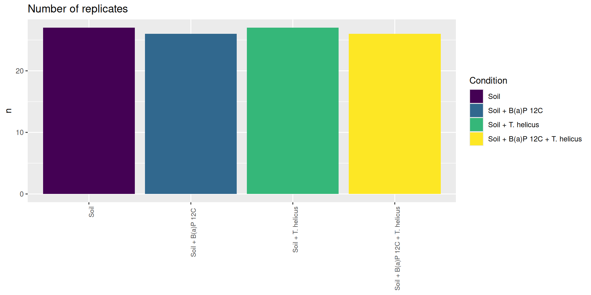
# count number of samples per conditionsample_data(physeq) %>%as_tibble() %>% dplyr::count(Condition)
# A tibble: 4 × 2
Condition n
<ord> <int>
1 "Soil" 27
2 "Soil + B(a)P 12C " 26
3 "Soil + T. helicus" 27
4 "Soil + B(a)P 12C + T. helicus" 26
Code
# library(magrittr)# sample_data(physeq) %$%# table(ConditionName, Incubation, Deep)sample_data(physeq) %>%as_tibble() %>% dplyr::add_count(Condition) %>% dplyr::select(Condition, n) %>%distinct() %>%ggplot(., aes(x = Condition, y = n, fill = Condition)) +geom_bar(stat ="identity") +labs(title="Number of replicates", y ="n") +theme(axis.title.x =element_blank(),axis.text.x =element_text(angle =90, size =8, hjust =1))
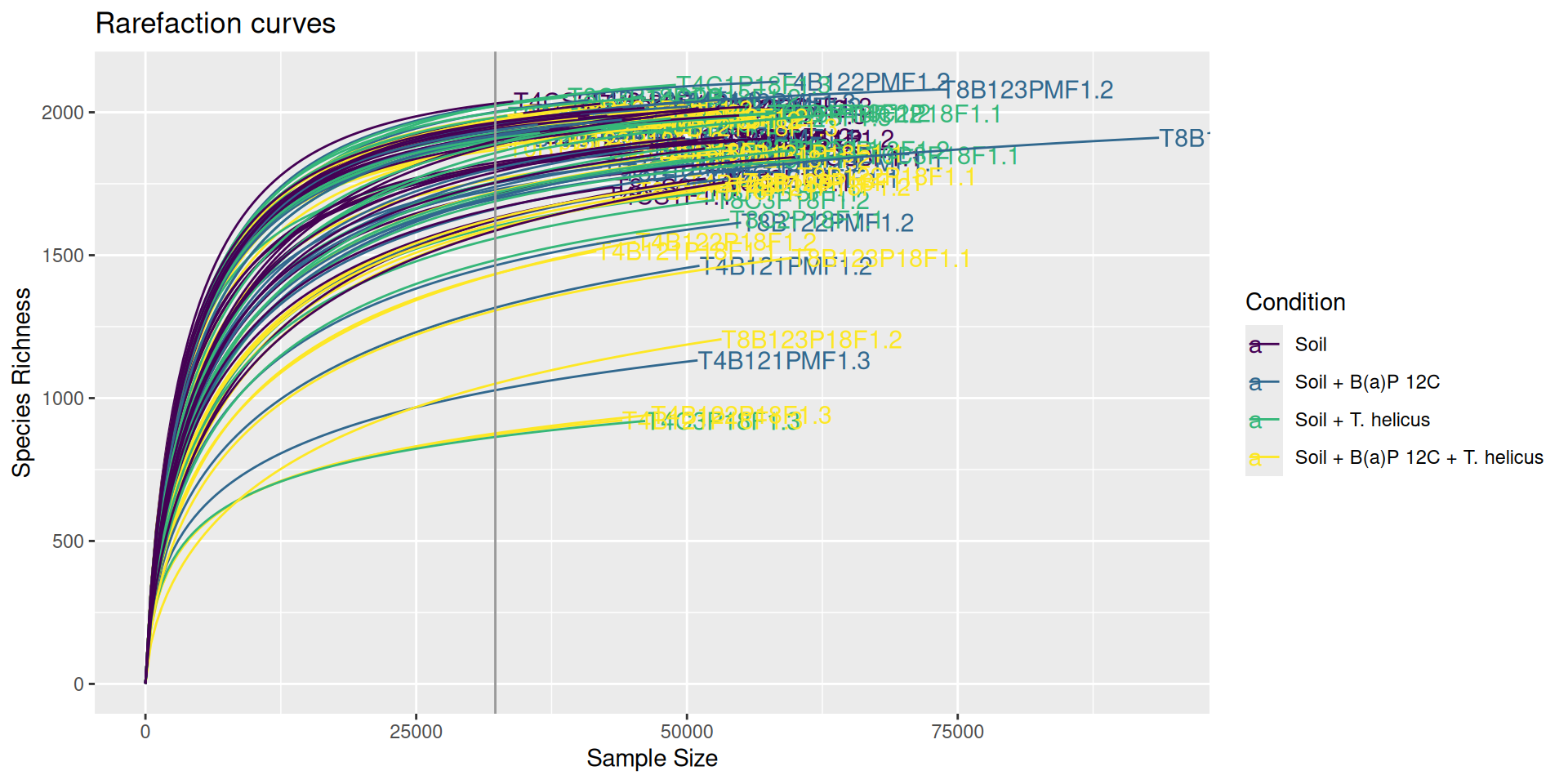
Rarefaction
The common practice for comparing microbiome samples of different library sizes is to reduce the size of the larger samples using rarefaction until they contain the same number of reads as the smallest sample. The rarefaction curves show the species richness (i.e. number of species) against the library size and the vertical grey line indicates the smallest sample’s size. Each curve indicates when the sampling depth is sufficient to achieve an acceptable number of species discoveries and when increasing the depth leads to the discovery of rarer species. Rarefied data are used to estimate and compare alpha and beta diversity across samples.
Problematic taxa
taxa Kingdom Phylum Class Order Family
Cluster_519 Cluster_519 Bacteria Firmicutes Bacilli Bacillales Bacillaceae
Genus rank
Cluster_519 Multi-affiliation 6
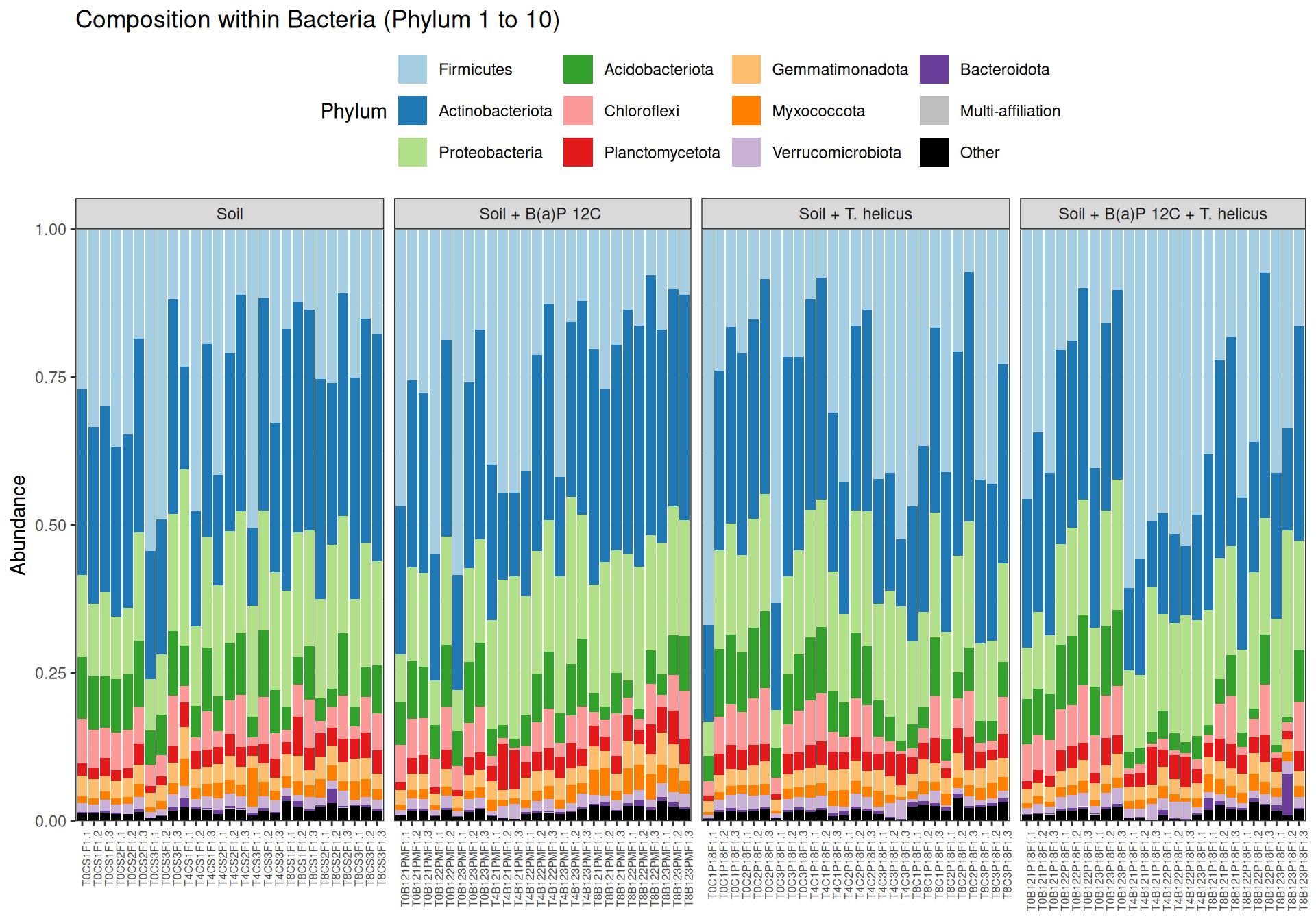
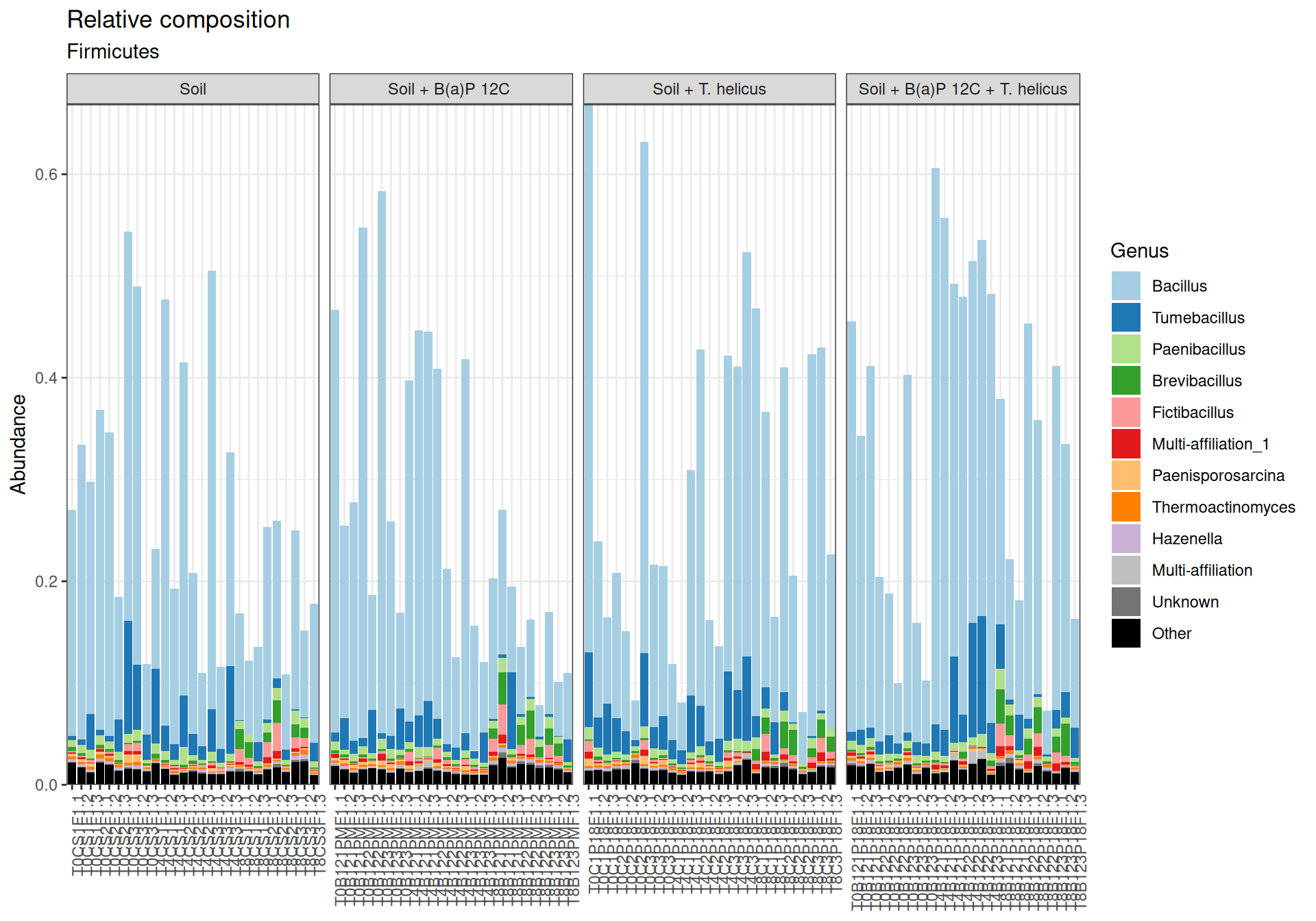
Bacillus, Tumebacillus genera are mainly representated in Firmicutes.
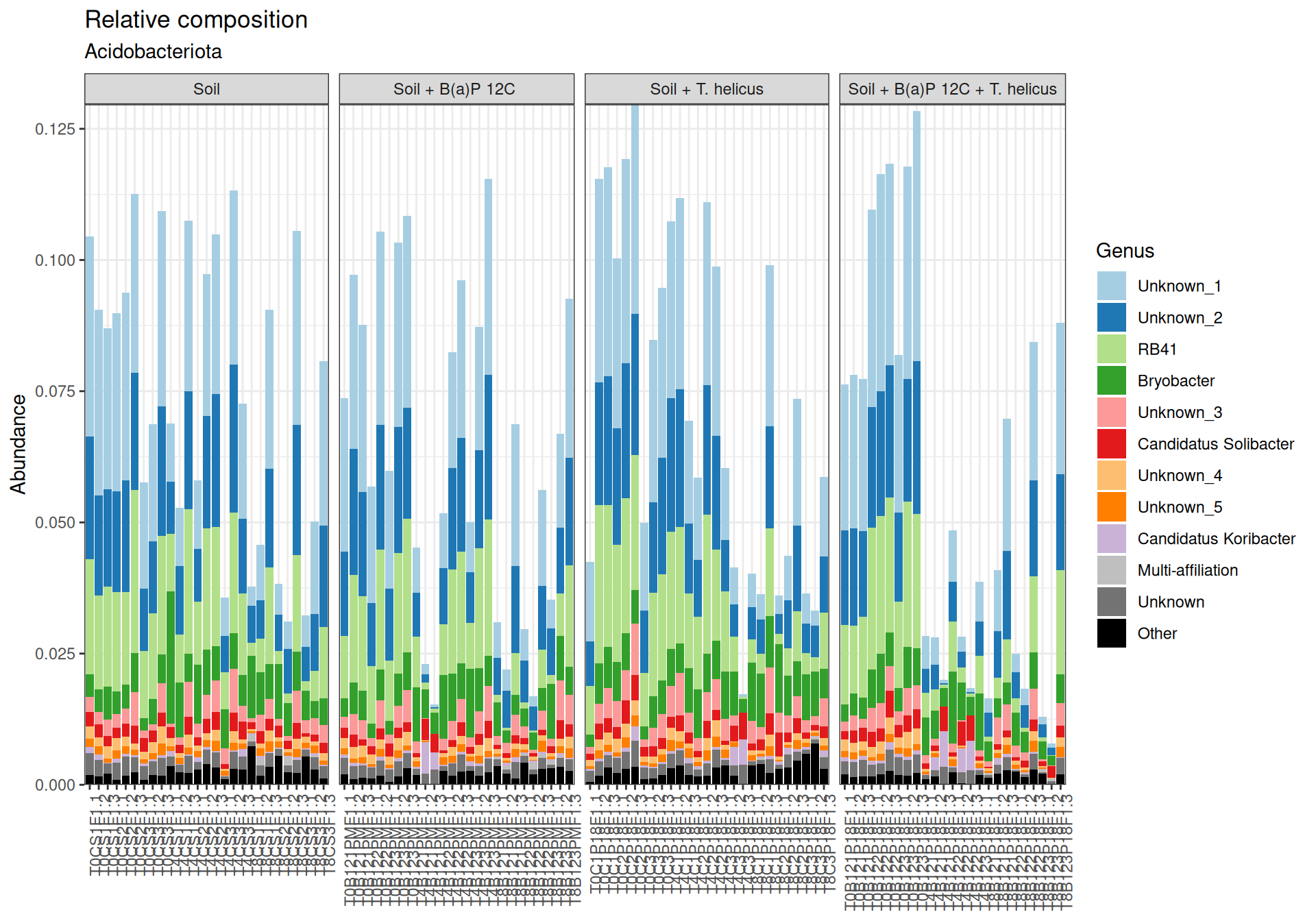
We note the presence of RB41, Bryobacter, Candidatus Solibacter and Candidatus Koribacter in Acidobacteriota phylum.
Alpha-diversity
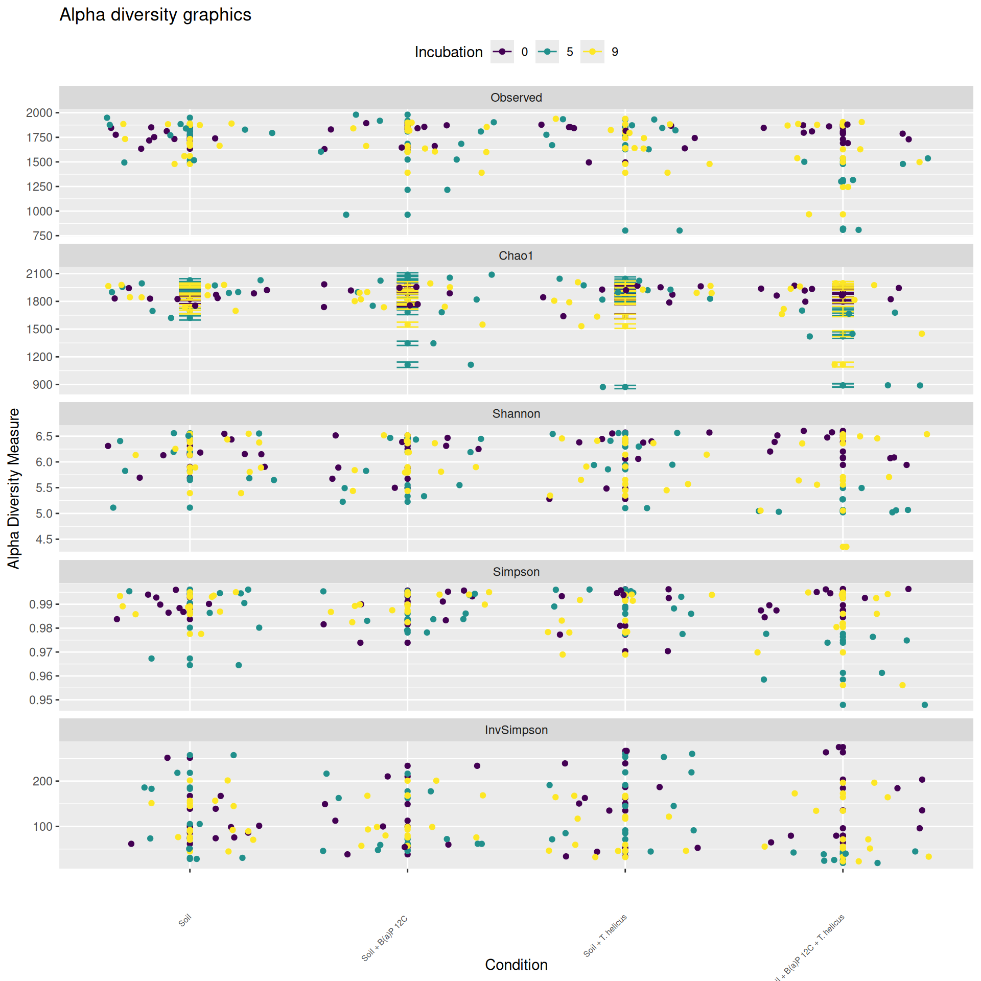
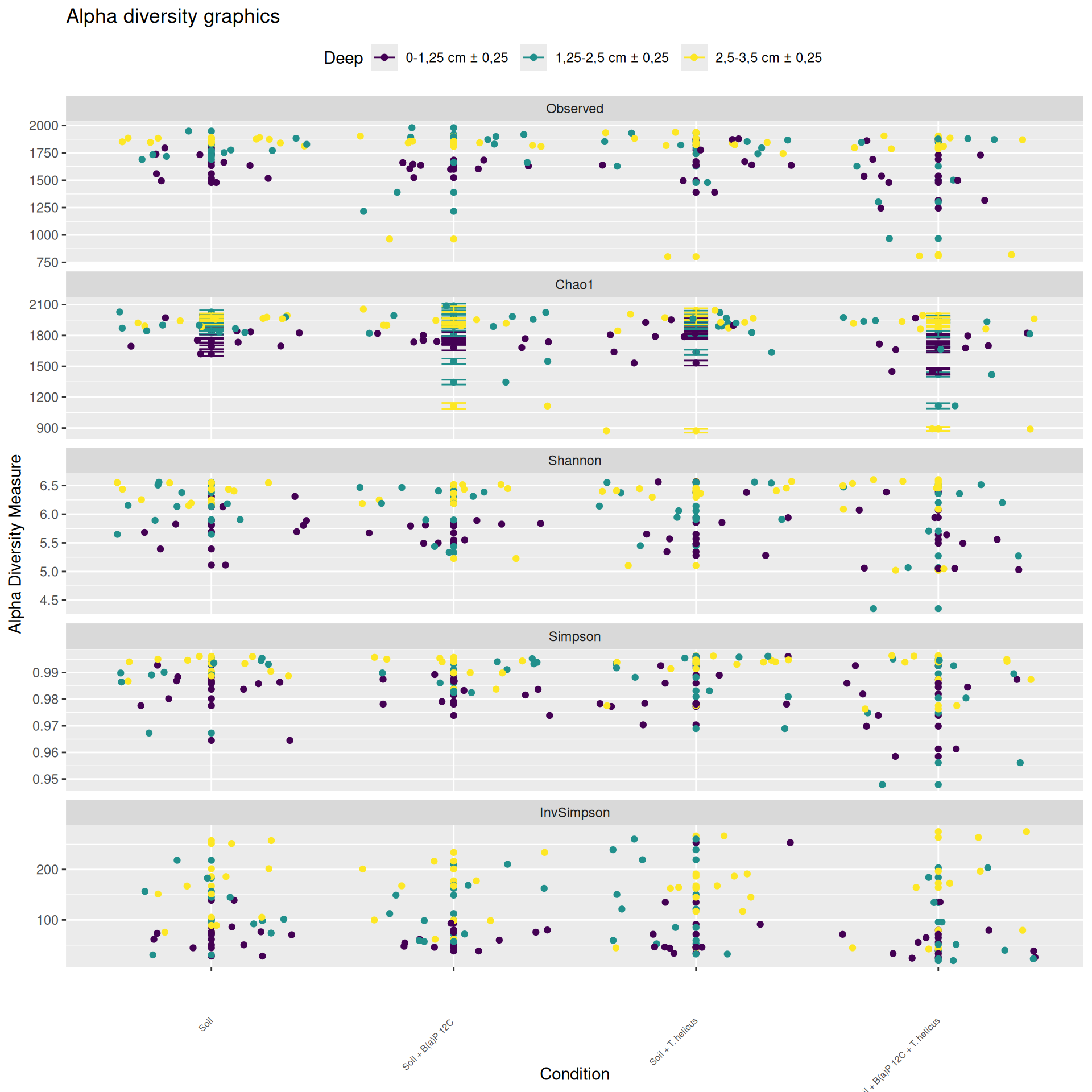
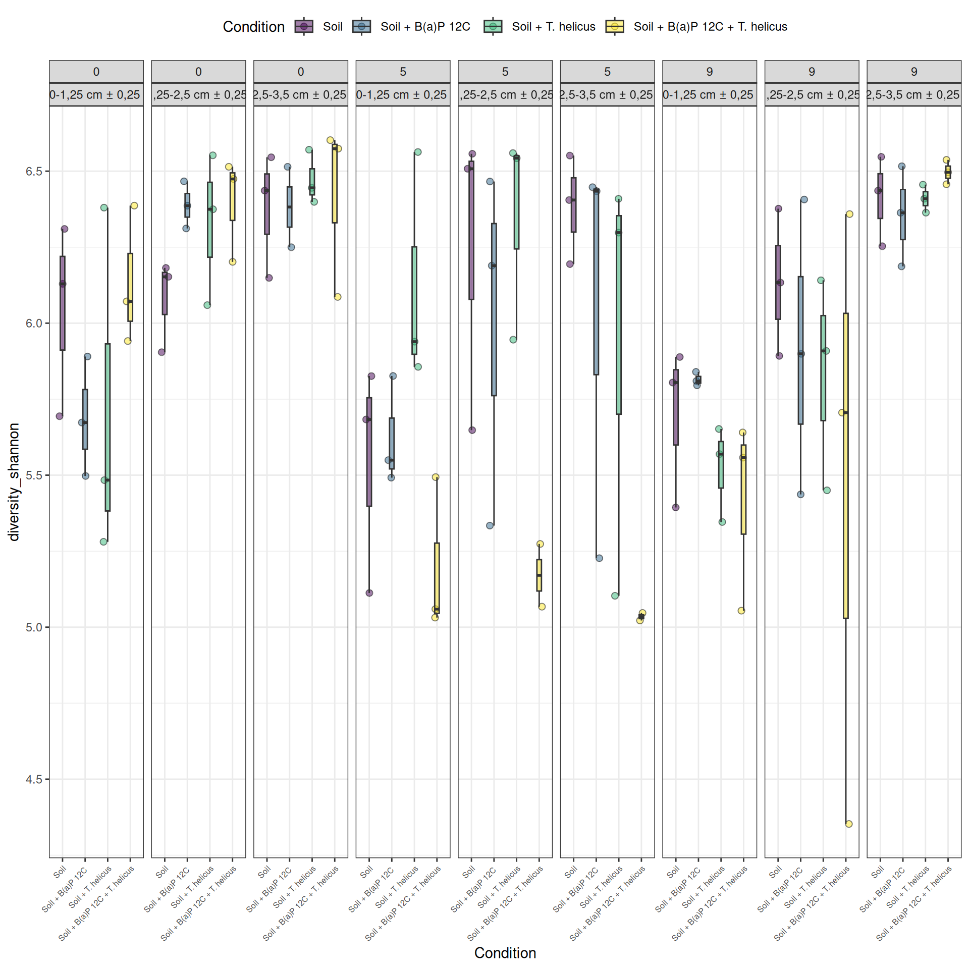
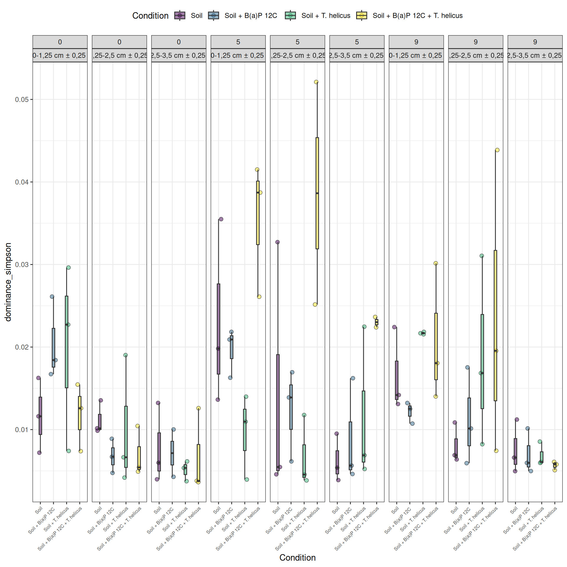
Alpha-diversity represents diversity within a sample. The most commonly used measures of diversity are : Observed, Chao1, Shannon, and Simpson. Richness (i.e. Observed) is simply the number of species present in the sample. Chao1 is an estimator of the number of species applied to the presence/absence data for each species. Shannon uses the abondance of different species and indicates richness and evenness. The Simpson index gives more importance to abundant species.
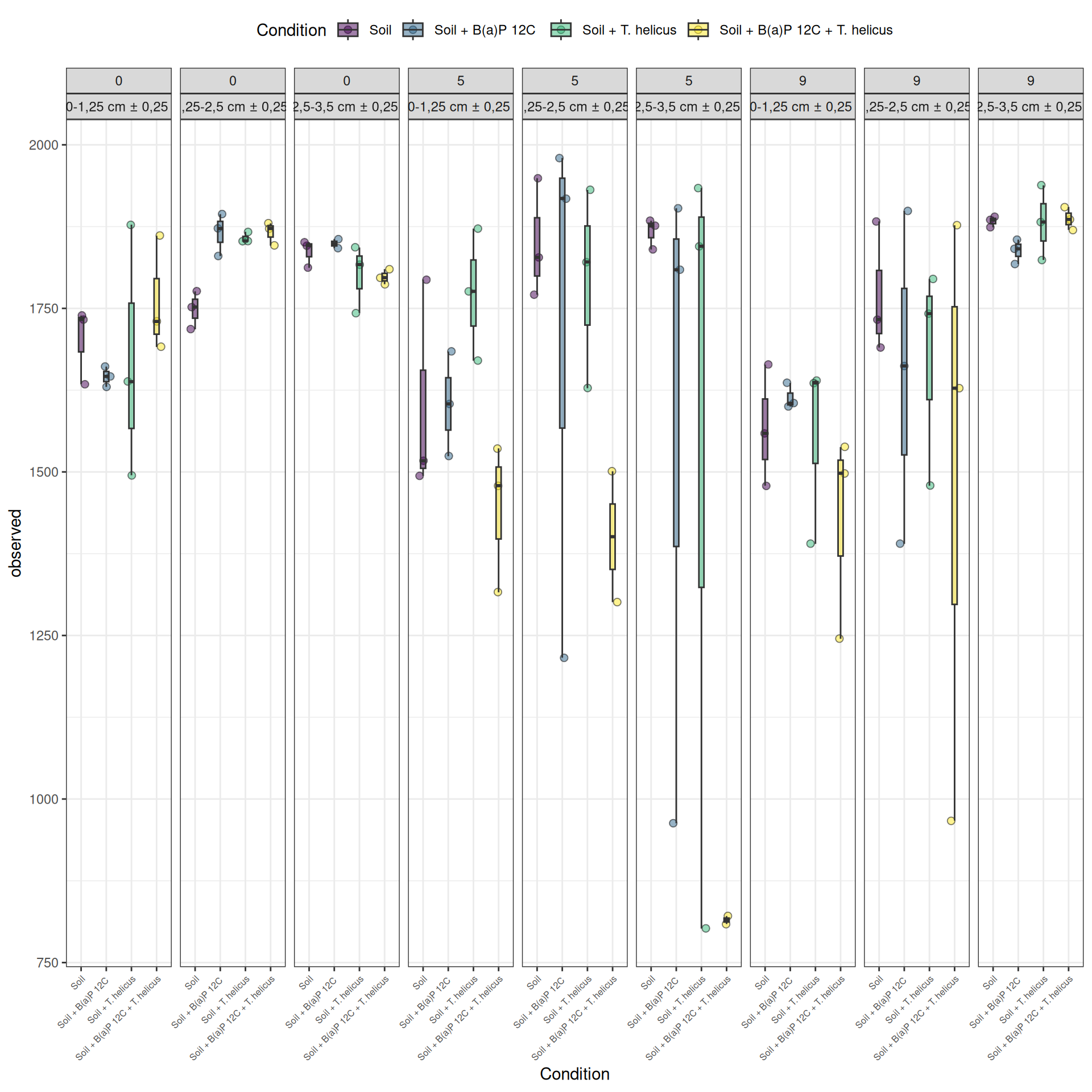
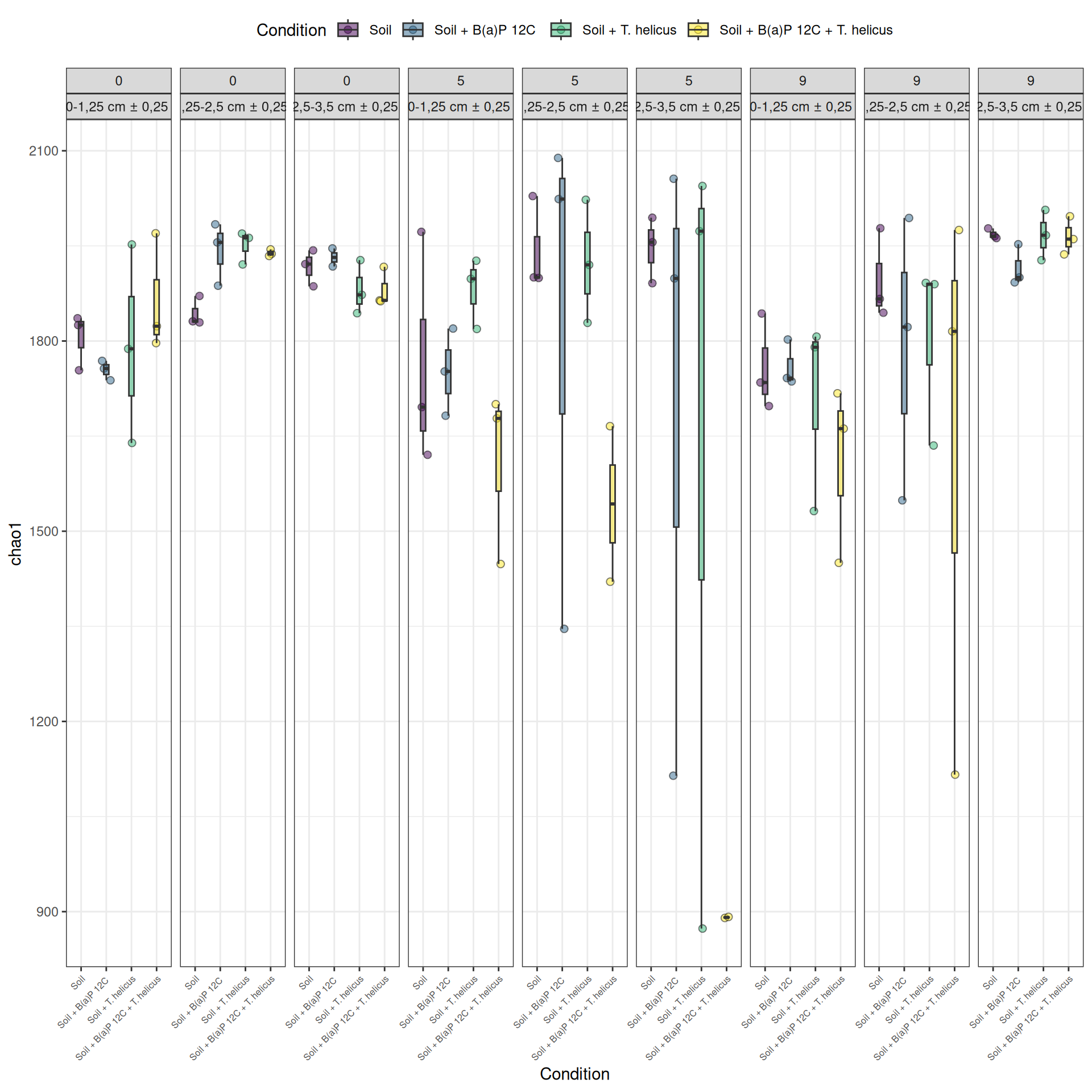
The soil samples collected at Incubation = 0 contain the highest homogeneous richness. The richness of the samples collected at Incubation = 9 and with a high value of Deep = 2,5-3,5 cm ± 0,25, is as high as at Incubation = 0. Some samples had low alpha diversity leading to high variablity for Condition = Soil + B(a)P 12C, incubation = 5, Deep = 2,5-3,5 cm ± 0,25, Condition = Soil + T. helicus, incubation = 5, Deep = 2,5-3,5 cm ± 0,25 and Condition = Soil + B(a)P 12C + T. helicus, incubation = 9, Deep = 1,25-2,5 cm ± 0,25.
Alpha-diversity - statistical tests
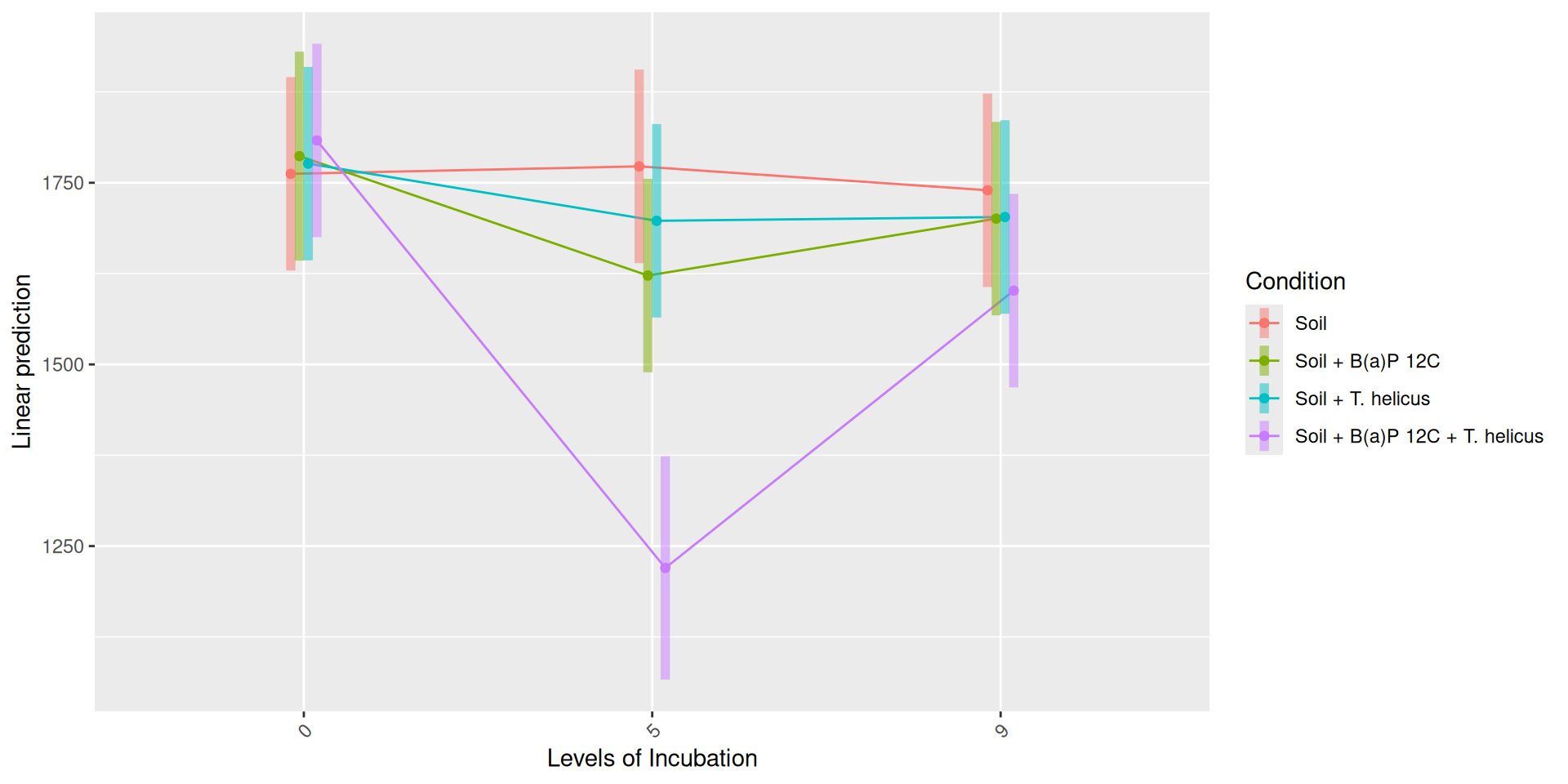
We calculated the alpha-diversity indices and combined them with covariates from experimental design. A linear model is fitted to test the influence of each factor and the interactions on the alpha-diversity (here, Observed measure).
#tests EMM <-emmeans(alphadiv.lm, ~ Condition*Incubation*Deep)# tests correction are performed within the variable# P value adjustment: tukey method for comparing comp1 <-pairs(EMM, simple ="Condition", adjust ="tukey")# P value adjustment: tukey method for comparing comp2 <-pairs(EMM, simple ="Incubation", adjust ="tukey")# P value adjustment: tukey method for comparing comp3 <-pairs(EMM, simple ="Deep", adjust ="tukey")
Results
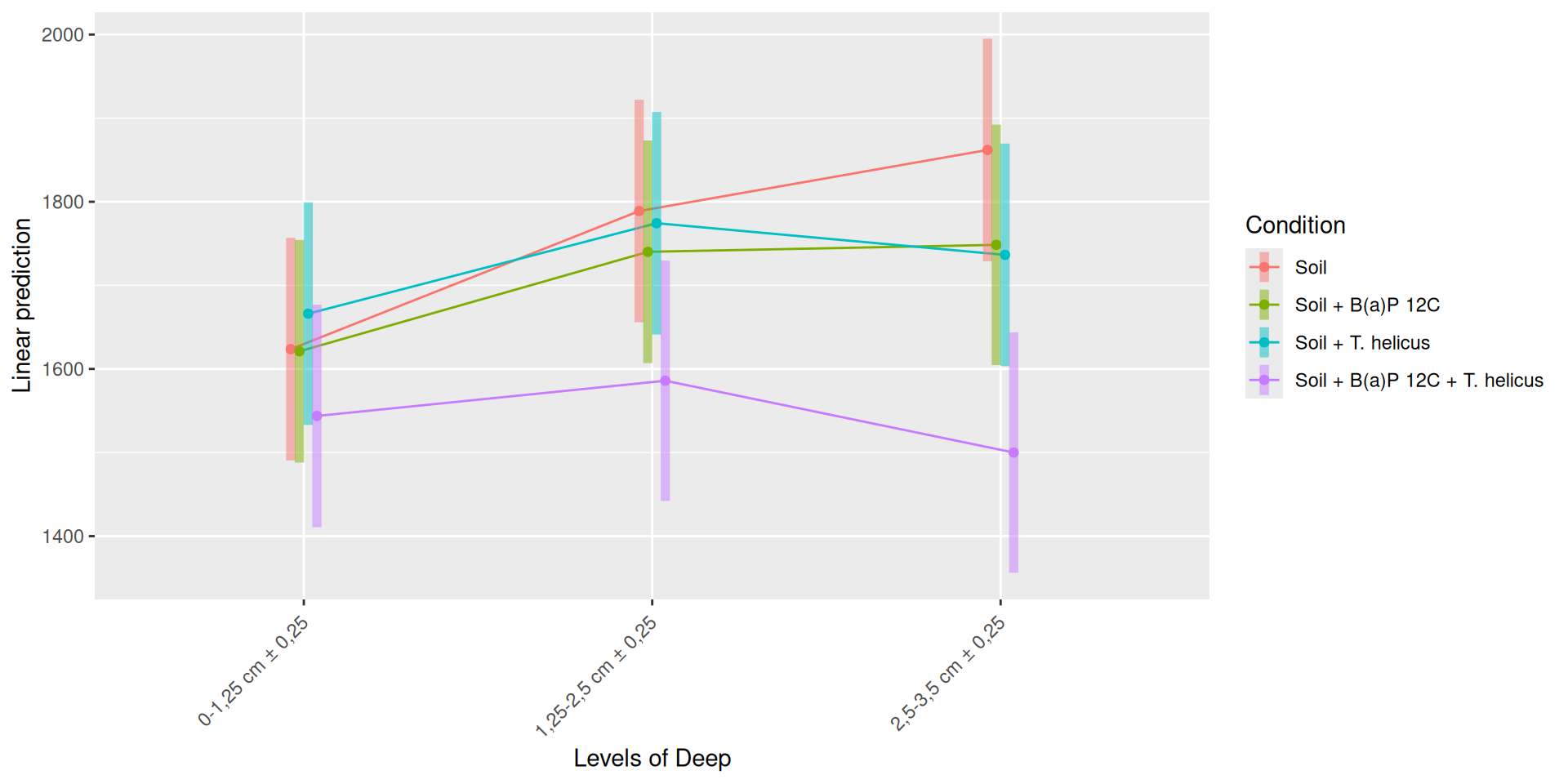
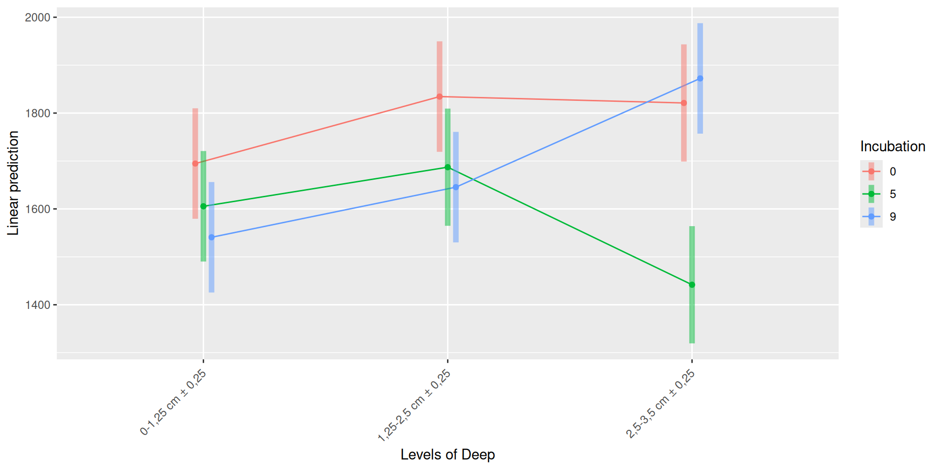
The richness (i.e. Observed index) is influenced by the interaction Condition:Incubation, Incubation:Deep. The simple effects of Condition, Incubation and Deep must be interpret with the interaction. Plots allow to visualize significant interactions at 0.05 Condition:Incubation and Incubation:Deep on rhe estimated marginal means fitted of the observed alpha-diversity. The interaction Condition:Deep is not significant but a lower diversity is shown for Soil + B(a)P 12C + T. helicus samples.
Pairwise tests between Condition and Incubation were performed with post hoc Tukey’s test to determine which were significant. These comparisons were significant at 0.05 (See downloads file):
Incubation = 5, Deep = 2,5-3,5 cm ± 0,25: Soil - (Soil + B(a)P 12C + T. helicus)
Soil + B(a)P 12C + T. helicus, Deep = 2,5-3,5 cm ± 0,25: Incubation0 - Incubation5
Soil + B(a)P 12C + T. helicus, Deep = 2,5-3,5 cm ± 0,25 : Incubation5 - Incubation9
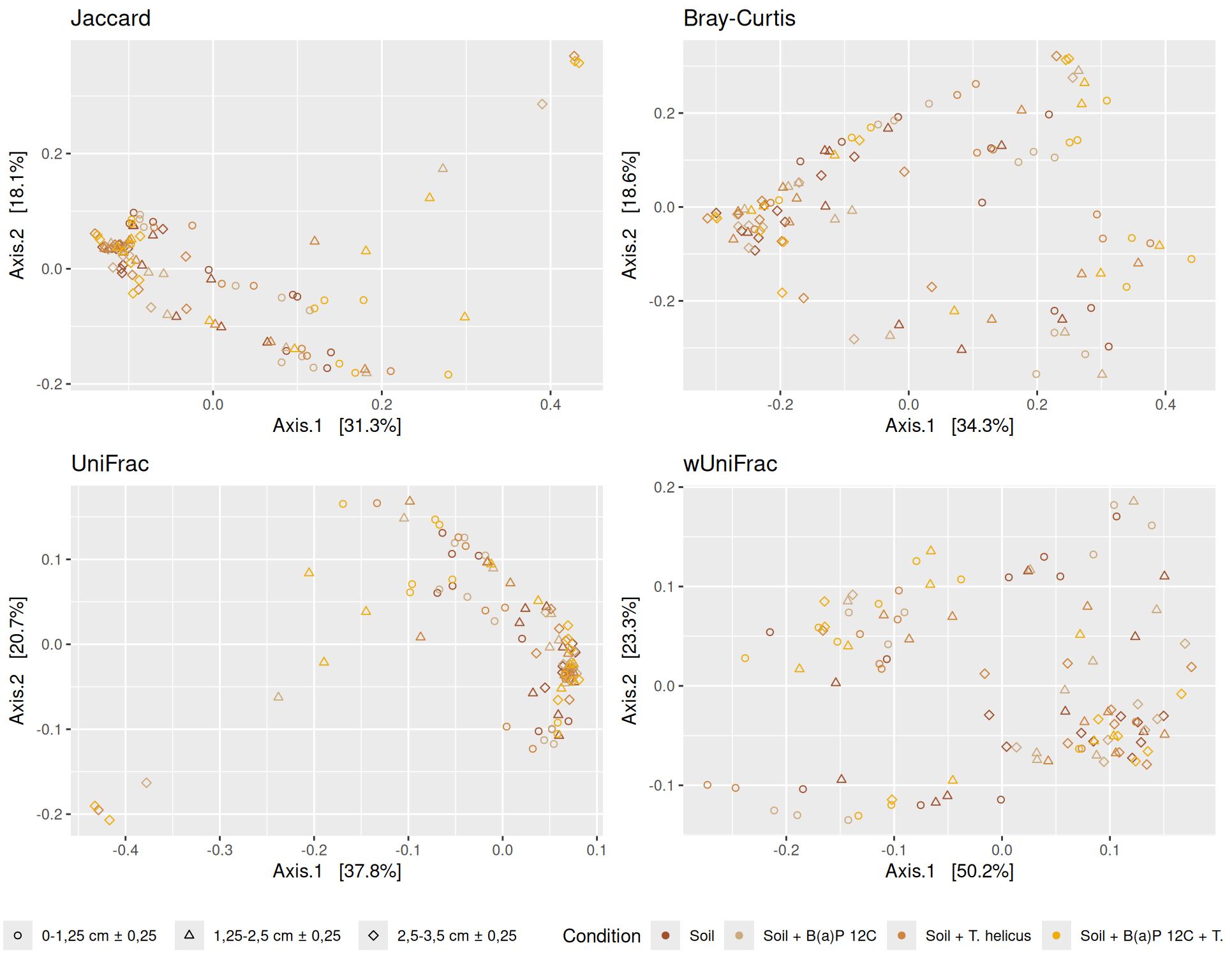
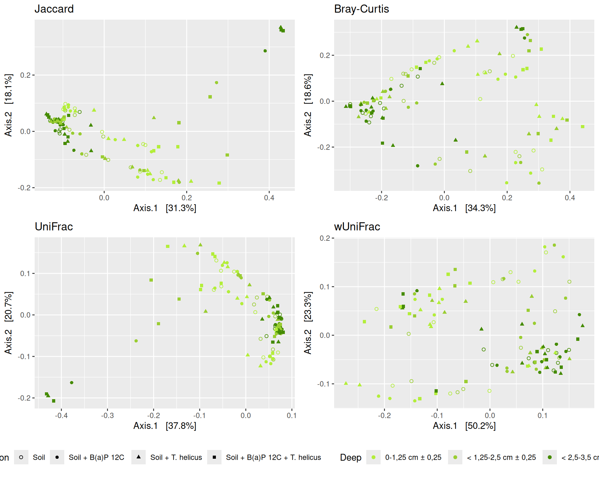
Beta-diversity
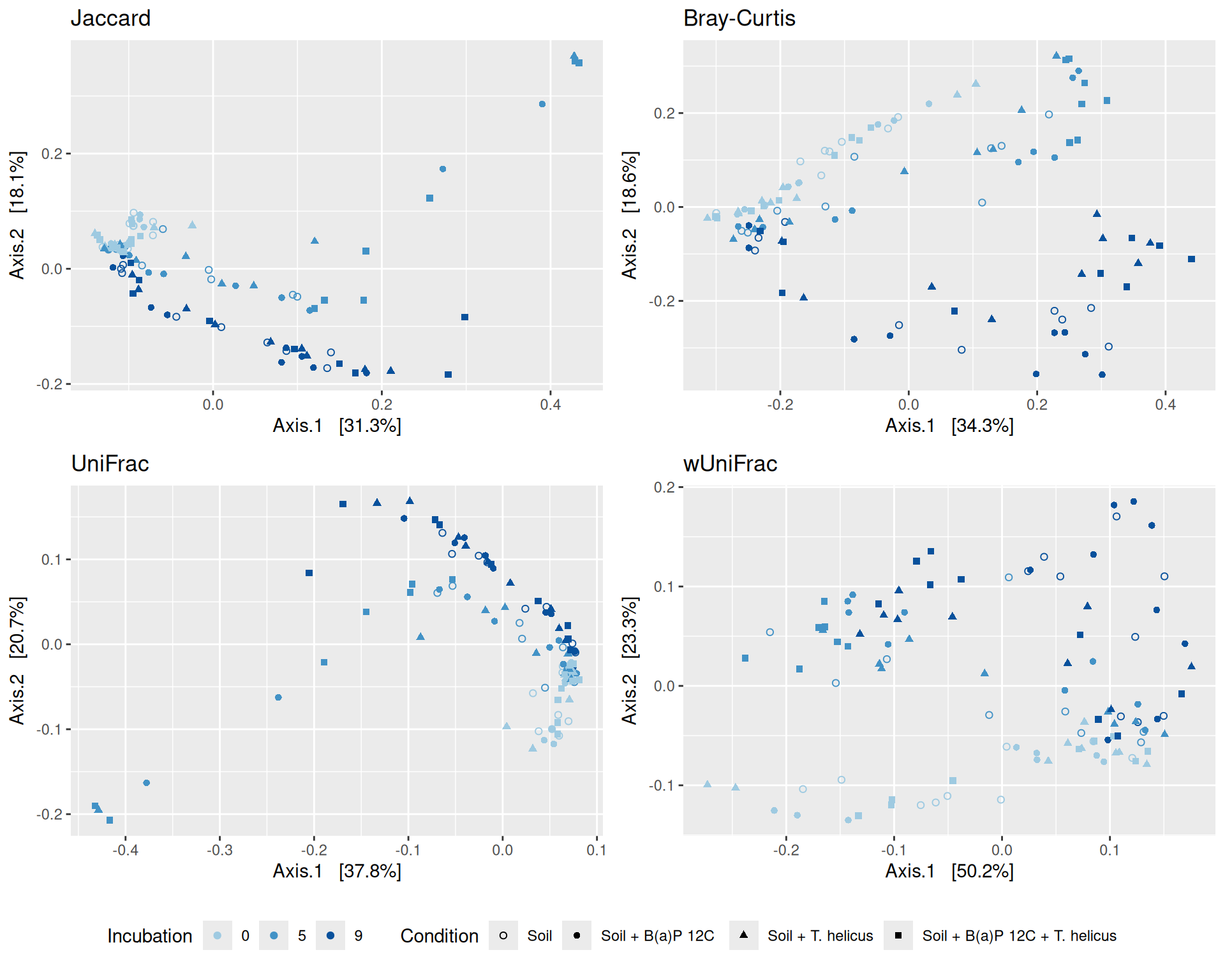
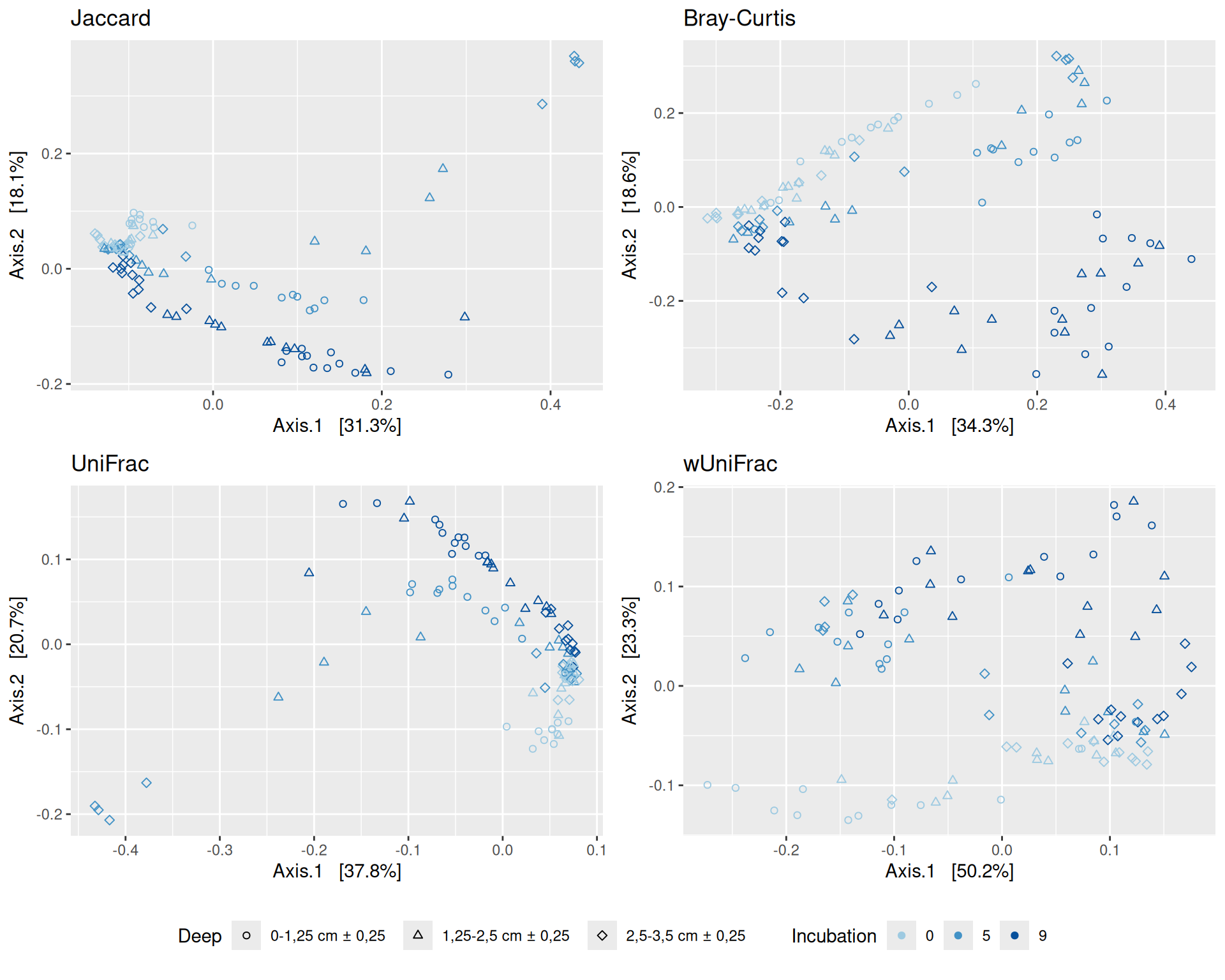
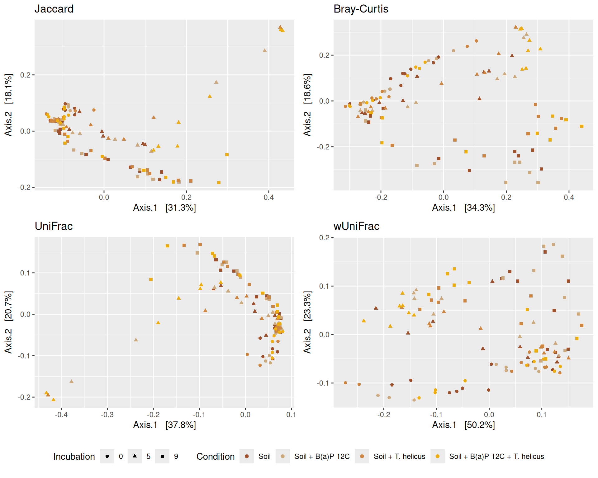
The dissimilarity between samples based on taxonomic composition is calculated with one of these Beta diversities: Bray-Curtis, Unweighted and weighted Unifrac, Jaccard index. The Bray-Curtis dissimilarity is calculated on counts and takes the value 0 when the composition of the samples est identical and the value 1 when the samples are completely disjoint. The Jaccard index uses presence/absence information only whereas UniFrac integrates information from the phylogenetic tree.
Here, we focused on the Multidimensional scaling (MDS / PCoA) based on Bray-Curtis distance and highlighted the effects of two significant interactions.
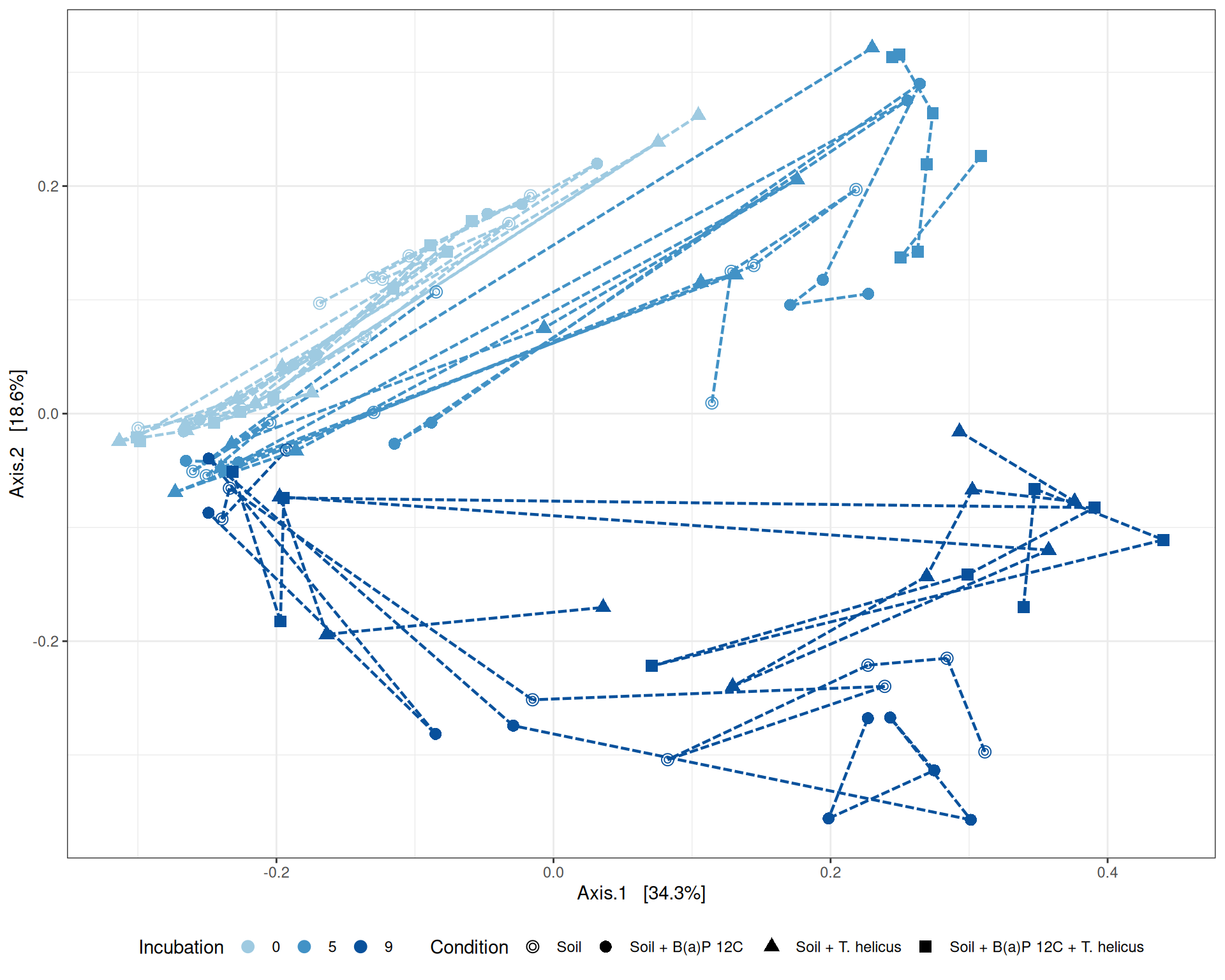
# MDS plot with arrows# effet le plus significatif est incubationp <-my_pcoa_with_arrows2(variable1 ="Incubation",variable2 ="Condition",physeq = physeq_rare,shapeval = Condition_shape$values,colorpal = Incubation_pal)p
Code
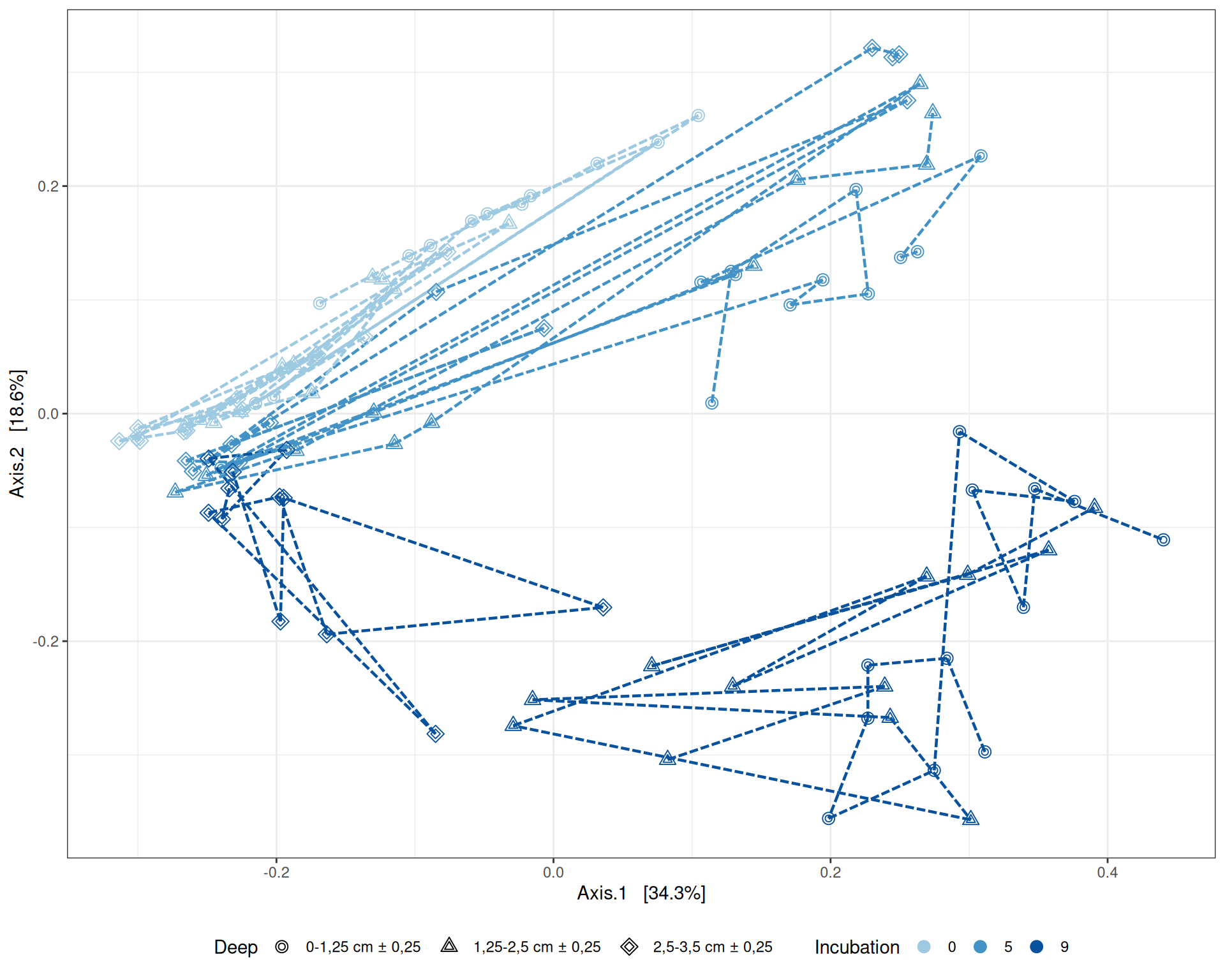
# MDS plot with arrows# effet le plus significatif est incubationp <-my_pcoa_with_arrows2(variable1 ="Incubation",variable2 ="Deep",physeq = physeq_rare,shapeval = Deep_shape$values,colorpal = Incubation_pal)p
MDS plot
The Multidimensional scaling (MDS / PCoA) based on Bray-Curtis distance showed that samples were firstly structured according to Incubation as the most significant variable in the alpha-diversity test. Different graphs help to visualize the effects of the interactions between Condition, Incubation and Deep.
Beta-diversity - Tests
Code
metadata <-sample_data(physeq_rare) %>%as("data.frame")# model <- vegan::adonis2(dist.bc ~ Condition*Incubation*Deep, data = metadata, permutations = 9999)# print(model)model <- vegan::adonis2(dist.bc ~ Incubation + Condition + Deep + Incubation:Condition + Incubation:Deep + Condition:Deep, data = metadata, permutations =9999)print(model)
Permutation test for adonis under reduced model
Permutation: free
Number of permutations: 9999
vegan::adonis2(formula = dist.bc ~ Incubation + Condition + Deep + Incubation:Condition + Incubation:Deep + Condition:Deep, data = metadata, permutations = 9999)
Df SumOfSqs R2 F Pr(>F)
Model 23 8.9447 0.60512 5.3967 1e-04 ***
Residual 81 5.8370 0.39488
Total 104 14.7817 1.00000
---
Signif. codes: 0 '***' 0.001 '**' 0.01 '*' 0.05 '.' 0.1 ' ' 1
Results
The change in microbiota composition measured by the Bray-Curtis Beta diversity is not significant for the interaction Condition*Incubation*Deep (not shown). So, the model was fitted without it. All effects were significant except for Condition:Deep at 0.05 significance level.
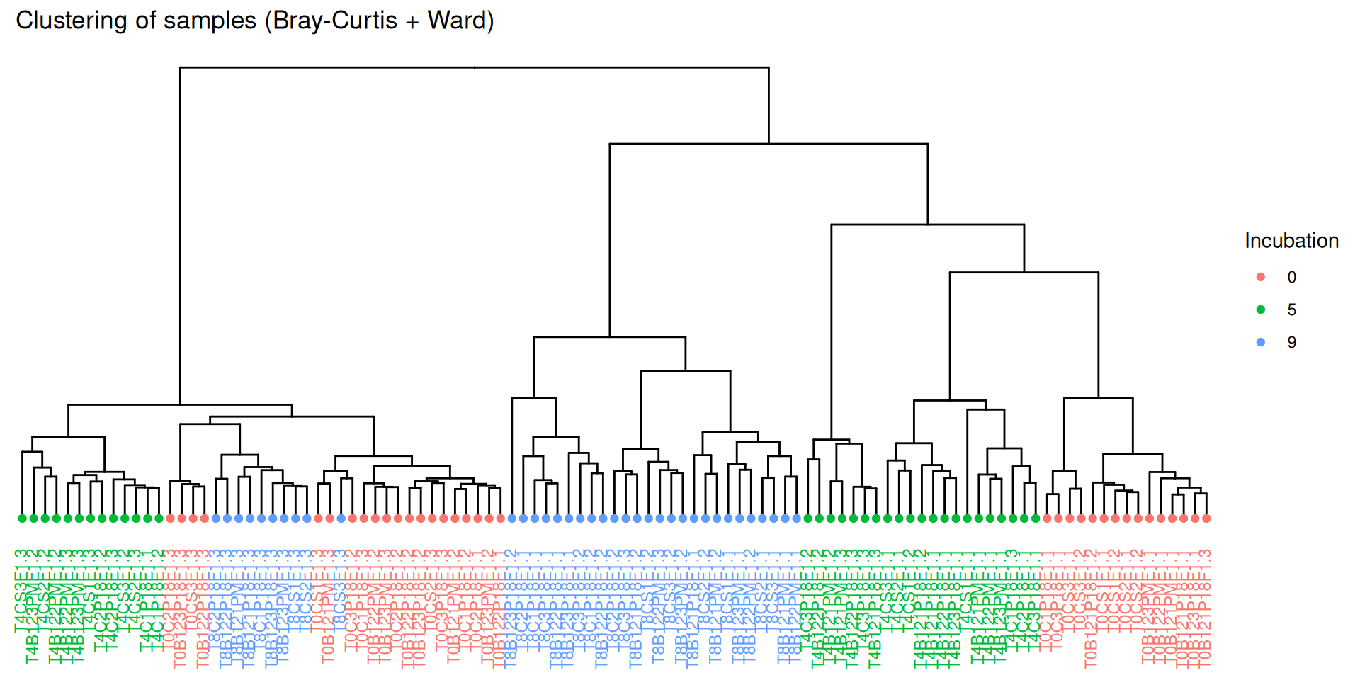
par(mar =c(3, 0, 2, 0), cex =0.6)phyloseq.extended::plot_clust(physeq_rare, dist ="bray", method ="ward.D2", color ="Incubation",title ="Clustering of samples (Bray-Curtis + Ward)")
Code
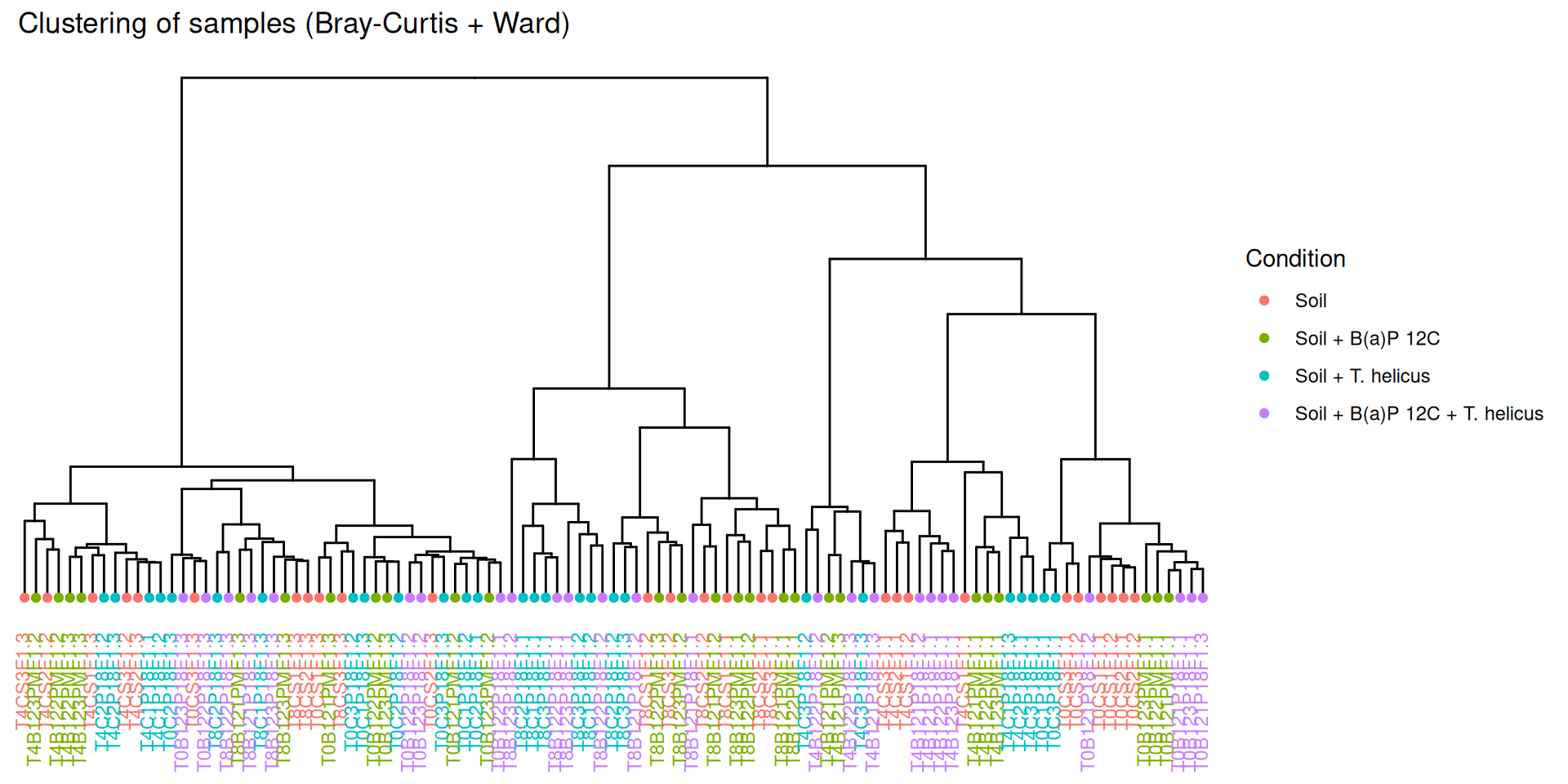
par(mar =c(3, 0, 2, 0), cex =0.6)phyloseq.extended::plot_clust(physeq_rare, dist ="bray", method ="ward.D2", color ="Condition",title ="Clustering of samples (Bray-Curtis + Ward)")
Code
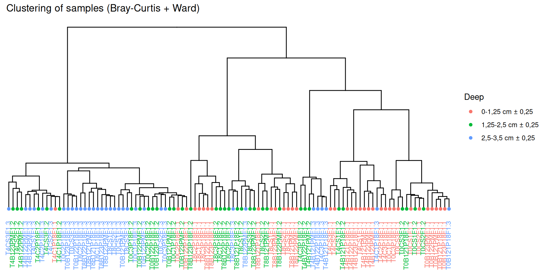
par(mar =c(3, 0, 2, 0), cex =0.6)phyloseq.extended::plot_clust(physeq_rare, dist ="bray", method ="ward.D2", color ="Deep",title ="Clustering of samples (Bray-Curtis + Ward)")
Results
Hierarchical clustering based on the Bray-Curtis dissimilarity and the Ward aggregation criterion shows that sample composition is not entirely structured by one of the factors Condition, Incubation and Deep due to the interactions. However, as previous results have shown, structuring is best explained by Incubation.
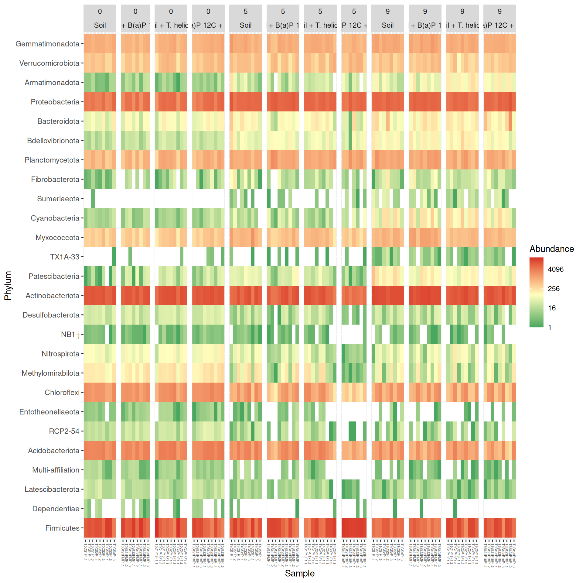
Heatmap using ordination
At Phylum taxonomic levels, we created heatmap plot of abundances using ordination methods to organize the rows with Bray-Curtis dissimilarity and Multidimensional scaling (MDS).
Code
# method = NULL if not ordinationp <- phyloseq::plot_heatmap(tax_glom(physeq_rare, taxrank="Phylum"), method ="MDS",distance ="bray",sample.order="SampleName", # not ordinationtaxa.label ="Phylum") +facet_grid(~ Incubation + Condition, scales ="free_x", space ="free_x") +scale_fill_gradient2(low ="#1a9850", mid ="#ffffbf", high ="#d73027",na.value ="white", trans = scales::log_trans(4),midpoint =log(100, base =4))p
Differential abundance analysis
The abundances data was not rarefied to performed differential abundance analysis. We are interested to identify taxa that were differentially abundant between Condition at Deepand Incubation fixed.
For convenience, the levels Soil, Soil + B(a)P 12C, Soil + T. helicus, Soil + B(a)P 12C + T. helicus, of the Condition factor have been relabelled as Soil, Soil_12C, Soil_heli, Soil_12C_heli, respectively. And the levels of 0-1,25 cm ± 0,25, 1,25-2,5 cm ± 0,25, 2,5-3,5 cm ± 0,25 of Deep factor have been relabelled as L, M, H, respectively.
phyloseq-class experiment-level object
otu_table() OTU Table: [ 2258 taxa and 105 samples ]
sample_data() Sample Data: [ 105 samples by 7 sample variables ]
tax_table() Taxonomy Table: [ 2258 taxa by 7 taxonomic ranks ]
phy_tree() Phylogenetic Tree: [ 2258 tips and 2257 internal nodes ]
Calculate the minimum number of replicates per Group.
Code
# calculate the minimum number of replicatesminreplicates <-sample_data(physeqbis) %>%as_tibble() %>% dplyr::add_count(Group) %>% dplyr::select(Group, n) %>% dplyr::summarise( min_nbreplicates =min(n))minreplicates
# A tibble: 1 × 1
min_nbreplicates
<int>
1 2
Code
# from Mahendra's functions# useful functions to perform a differential abundance analysis (daa)# filter taxa all zeros in all samples and # keep taxa with counts > 10 in at least the number of replicates - possibility to choosemy_filter_phyloseq <-function(physeq, nreplicates = minreplicates) { ii <- phyloseq::genefilter_sample(physeq, function(x) x >10, nreplicates) phyloseq::prune_taxa(ii, physeq)}# realise differential abundance results (daa) for the contrast# Note to specify a contrast as a listmy_extract_results <-function(deseq, test ="Wald", contrast) { DESeq2::results(deseq, test = test, tidy =TRUE, contrast = contrast) %>% dplyr::rename(ASV = row) %>%# dplyr::filter(padj <= 0.05) %>% dplyr::arrange(log2FoldChange)}# formatting the daa result by adding ASV informations into daa objectmy_format_results <-function(data, physeq) { phyloseq::tax_table(physeq)@.Data %>%as_tibble() %>%mutate(ASV =rownames(phyloseq::tax_table(physeq)@.Data)) %>% dplyr::right_join(., data, by ="ASV") %>%mutate(ASV =factor(ASV, levels = data$ASV))}# combine my_extract_results and my_format_results into an unique function# realise differential abundance results (daa) for the contrast# Note to specify a contrast as a listmy_daa_results <-function(deseq, test ="Wald", physeq, contrast) {# provide differential abundance results (daa) for the contrast# sort by log2FoldChange daa <- DESeq2::results(deseq, test = test, tidy =TRUE, contrast = contrast) %>% dplyr::rename(ASV = row) %>% dplyr::filter(padj <=0.05) # add ASV informations into daa object daa_new <- phyloseq::tax_table(physeq)@.Data %>%as_tibble() %>%mutate(ASV =rownames(phyloseq::tax_table(physeq)@.Data)) %>% dplyr::right_join(., daa, by ="ASV") %>%mutate(ASV =factor(ASV, levels = daa$ASV)) %>% dplyr::arrange(log2FoldChange)return(daa_new)}
phyloseq-class experiment-level object
otu_table() OTU Table: [ 373 taxa and 105 samples ]
sample_data() Sample Data: [ 105 samples by 7 sample variables ]
tax_table() Taxonomy Table: [ 373 taxa by 7 taxonomic ranks ]
phy_tree() Phylogenetic Tree: [ 373 tips and 372 internal nodes ]
Differential abundance analysis
The differential abundance analysis (DAA) is based on a Generalized Linear Model (GLM) to take into account the distribution of count-type data (non-normality of the data) and over-dispersion. The regression coefficients of the factors are estimated in the model and Wald test was used to identify DAA ASV’s in a defined contrast.
Using DESeq2 R package, the GLM model [3] was fitted with one factor combining the factors of interest. A Benjamini-Hochberg false discovery rate (FDR) correction [4] was applied on pvalues.
Code
# do not rarefy# at defined level taxrank# filtering low abundance: less 10 in at least nreplicatescds <- phyloseq::phyloseq_to_deseq2(physeq_filter,~0+ Group)SummarizedExperiment::rowData(cds) <- phyloseq::tax_table(physeq_filter)#rownames(SummarizedExperiment::colData(cds)) <- SummarizedExperiment::colData(cds)$SampleLabel# cds is a summarized experiment object SE# experimental design# colData(cds)# abundances# assays(cds)$counts# fit Negative Binomial GLM modeldds <- DESeq2::DESeq(cds, sfType ="poscounts", fitType='local', test="Wald")dds_coeff <- DESeq2::resultsNames(dds)
Differential abundance analysis between Condition
Code
# define interesting contrastscontrast_Condition <-list("H0_Soil_12C_vs_Soil"=c("GroupH_0_Soil_12C", "GroupH_0_Soil"),"H0_Soil_12C_heli_vs_Soil_heli"=c("GroupH_0_Soil_12C_heli", "GroupH_0_Soil_heli"),"H0_Soil_heli_vs_Soil"=c("GroupH_0_Soil_heli", "GroupH_0_Soil"),"H0_Soil_12C_heli_vs_Soil_12C"=c("GroupH_0_Soil_12C_heli", "GroupH_0_Soil_12C"),"H5_Soil_12C_vs_Soil"=c("GroupH_5_Soil_12C", "GroupH_5_Soil"),"H5_Soil_12C_heli_vs_Soil_heli"=c("GroupH_5_Soil_12C_heli", "GroupH_5_Soil_heli"),"H5_Soil_heli_vs_Soil"=c("GroupH_5_Soil_heli", "GroupH_5_Soil"),"H5_Soil_12C_heli_vs_Soil_12C"=c("GroupH_5_Soil_12C_heli", "GroupH_5_Soil_12C"),"H9_Soil_12C_vs_Soil"=c("GroupH_9_Soil_12C", "GroupH_9_Soil"),"H9_Soil_12C_heli_vs_Soil_heli"=c("GroupH_9_Soil_12C_heli", "GroupH_9_Soil_heli"),"H9_Soil_heli_vs_Soil"=c("GroupH_9_Soil_heli", "GroupH_9_Soil"),"H9_Soil_12C_heli_vs_Soil_12C"=c("GroupH_9_Soil_12C_heli", "GroupH_9_Soil_12C"),"M0_Soil_12C_vs_Soil"=c("GroupM_0_Soil_12C", "GroupM_0_Soil"),"M0_Soil_12C_heli_vs_Soil_heli"=c("GroupM_0_Soil_12C_heli", "GroupM_0_Soil_heli"),"M0_Soil_heli_vs_Soil"=c("GroupM_0_Soil_heli", "GroupM_0_Soil"),"M0_Soil_12C_heli_vs_Soil_12C"=c("GroupM_0_Soil_12C_heli", "GroupM_0_Soil_12C"),"M5_Soil_12C_vs_Soil"=c("GroupM_5_Soil_12C", "GroupM_5_Soil"),"M5_Soil_12C_heli_vs_Soil_heli"=c("GroupM_5_Soil_12C_heli", "GroupM_5_Soil_heli"),"M5_Soil_heli_vs_Soil"=c("GroupM_5_Soil_heli", "GroupM_5_Soil"),"M5_Soil_12C_heli_vs_Soil_12C"=c("GroupM_5_Soil_12C_heli", "GroupM_5_Soil_12C"),"M9_Soil_12C_vs_Soil"=c("GroupM_9_Soil_12C", "GroupM_9_Soil"),"M9_Soil_12C_heli_vs_Soil_heli"=c("GroupM_9_Soil_12C_heli", "GroupM_9_Soil_heli"),"M9_Soil_heli_vs_Soil"=c("GroupM_9_Soil_heli", "GroupM_9_Soil"),"M9_Soil_12C_heli_vs_Soil_12C"=c("GroupM_9_Soil_12C_heli", "GroupM_9_Soil_12C"),"L0_Soil_12C_vs_Soil"=c("GroupL_0_Soil_12C", "GroupL_0_Soil"),"L0_Soil_12C_heli_vs_Soil_heli"=c("GroupL_0_Soil_12C_heli", "GroupL_0_Soil_heli"),"L0_Soil_heli_vs_Soil"=c("GroupL_0_Soil_heli", "GroupL_0_Soil"),"L0_Soil_12C_heli_vs_Soil_12C"=c("GroupL_0_Soil_12C_heli", "GroupL_0_Soil_12C"),"L5_Soil_12C_vs_Soil"=c("GroupL_5_Soil_12C", "GroupL_5_Soil"),"L5_Soil_12C_heli_vs_Soil_heli"=c("GroupL_5_Soil_12C_heli", "GroupL_5_Soil_heli"),"L5_Soil_heli_vs_Soil"=c("GroupL_5_Soil_heli", "GroupL_5_Soil"),"L5_Soil_12C_heli_vs_Soil_12C"=c("GroupL_5_Soil_12C_heli", "GroupL_5_Soil_12C"),"L9_Soil_12C_vs_Soil"=c("GroupL_9_Soil_12C", "GroupL_9_Soil"),"L9_Soil_12C_heli_vs_Soil_heli"=c("GroupL_9_Soil_12C_heli", "GroupL_9_Soil_heli"),"L9_Soil_heli_vs_Soil"=c("GroupL_9_Soil_heli", "GroupL_9_Soil"),"L9_Soil_12C_heli_vs_Soil_12C"=c("GroupL_9_Soil_12C_heli", "GroupL_9_Soil_12C"))# realize a daa for a list of contrasts# list of differential analyses results for each contrast# daa_deseq2_Condition <- contrast_Condition |># map(\(x) my_extract_results(dds, contrast = list(x)))# daa_deseq2_Condition# extract result for a fixed contrast# daa_deseq2 <- my_extract_results(dds, contrast = list(contrast_Condition[[1]]))# format dda result for a fixed contrast# daa_res <- my_format_results(data = daa_deseq2, physeq = physeq_filter)# combine the previous functions# realize a differential abunbdance analyses (dda) for a list of contrasts# format dda: adding ASV informations and sorting by log2FoldChangedaa_deseq2_Condition <- contrast_Condition |>map(\(x) my_daa_results(dds, test ="Wald", physeq = physeq_filter, contrast =list(x))) #example for one contrast#res <- my_daa_results(dds, test = "Wald", contrast = list(contrast_Condition[[1]]), physeq = physeq_filter)
This is the number of differentially abundant ASV (at genus) obtained for each tested contrast: pairwise contrast between the levels of factor of interest.
Code
# number of taxomic group daa for each tested contrastdaa_deseq2_Condition |>map_df(nrow) |>t() |>kbl(col.names =c("Nb of diff. abundant ASV (at genus)")) |>kable_styling() |>scroll_box(height ="600px")
Nb of diff. abundant ASV (at genus)
H0_Soil_12C_vs_Soil
326
H0_Soil_12C_heli_vs_Soil_heli
326
H0_Soil_heli_vs_Soil
328
H0_Soil_12C_heli_vs_Soil_12C
323
H5_Soil_12C_vs_Soil
335
H5_Soil_12C_heli_vs_Soil_heli
221
H5_Soil_heli_vs_Soil
339
H5_Soil_12C_heli_vs_Soil_12C
226
H9_Soil_12C_vs_Soil
335
H9_Soil_12C_heli_vs_Soil_heli
339
H9_Soil_heli_vs_Soil
334
H9_Soil_12C_heli_vs_Soil_12C
334
M0_Soil_12C_vs_Soil
318
M0_Soil_12C_heli_vs_Soil_heli
332
M0_Soil_heli_vs_Soil
321
M0_Soil_12C_heli_vs_Soil_12C
333
M5_Soil_12C_vs_Soil
343
M5_Soil_12C_heli_vs_Soil_heli
307
M5_Soil_heli_vs_Soil
340
M5_Soil_12C_heli_vs_Soil_12C
305
M9_Soil_12C_vs_Soil
337
M9_Soil_12C_heli_vs_Soil_heli
324
M9_Soil_heli_vs_Soil
329
M9_Soil_12C_heli_vs_Soil_12C
335
L0_Soil_12C_vs_Soil
314
L0_Soil_12C_heli_vs_Soil_heli
323
L0_Soil_heli_vs_Soil
307
L0_Soil_12C_heli_vs_Soil_12C
306
L5_Soil_12C_vs_Soil
317
L5_Soil_12C_heli_vs_Soil_heli
320
L5_Soil_heli_vs_Soil
323
L5_Soil_12C_heli_vs_Soil_12C
306
L9_Soil_12C_vs_Soil
319
L9_Soil_12C_heli_vs_Soil_heli
312
L9_Soil_heli_vs_Soil
307
L9_Soil_12C_heli_vs_Soil_12C
326
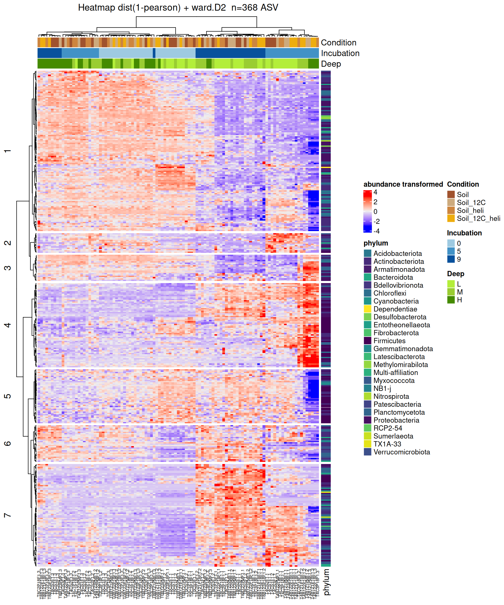
Heatmap based on Condition contrasts
Heatmap
After the differential abundance analysis, a hierarchical clustering followed by a heatmap plot [5] were performed on DA ASV in at least one of the comparisons, with ComplexHeatmap R package.
Abundances matrix was transformed using vst function from DESeq2 R package to stabilize the variance and take into account for sequencing bias. Rows (=ASV) were centered and divided by the standard deviation.
Hierarchical clustering was performed for both rows and columns in two steps: 1/ calculate the pearson distance (1 - corr) and 2/ apply a clustering method with the Ward’s distance.
Code
#vector containing DAA ASV in at least one of contrastdaa_asv <- daa_deseq2_Condition |>map_df(\(x) dplyr::select(x, ASV)) |>t() |>as.character() |>unique()
Code
# abundances were agglomerated by rank = Genus# calculate a variance stabilizing transformation VST# rows (= ASV) were centered and scaled vsd <- DESeq2::varianceStabilizingTransformation(dds, fitType="local", blind =FALSE)SummarizedExperiment::assay(vsd) <- SummarizedExperiment::assay(vsd)|>t() |>scale(center =TRUE, scale =TRUE) |>t()# select daa ASVvsd <- vsd[daa_asv,]#colData(vsd)#assay(vsd)#assay(vsd)["Cluster_xxx",]
The clustering revealed 7 groups of DA ASV between Condition contrasts that share the same abundance profile. As explained by previous analyses, the profiles are mainly characterized by Incubation. The samples were not clustered by Condition. Then, within a group, profiles are interpreted on the basis of striking samples corresponding to combinations of interest in the 3 factors. Please note: the number of groups has been set arbitrarily on the basis of dendrogram visualization.
This is the number of differentially abundant ASV (at genus) obtained for each tested contrast: pairwise contrast between the levels of factor of interest.
Code
# number of taxomic group daa for each tested contrastdaa_deseq2_Incubation|>map_df(nrow) |>t() |>kbl(col.names =c("Nb of diff. abundant ASV (at genus)")) |>kable_styling() |>scroll_box(height ="600px")
Nb of diff. abundant ASV (at genus)
H_Soil_9vs5
330
H_Soil_5vs0
333
H_Soil_9vs0
335
H_Soil_12C_9vs5
335
H_Soil_12C_5vs0
329
H_Soil_12C_9vs0
329
H_Soil_heli_9vs5
340
H_Soil_heli_5vs0
339
H_Soil_heli_9vs0
331
H_Soil_12C_heli_9vs5
230
H_Soil_12C_heli_5vs0
230
H_Soil_12C_heli_9vs0
328
M_Soil_9vs5
339
M_Soil_5vs0
325
M_Soil_9vs0
321
M_Soil_12C_9vs5
340
M_Soil_12C_5vs0
339
M_Soil_12C_9vs0
337
M_Soil_heli_9vs5
339
M_Soil_heli_5vs0
339
M_Soil_heli_9vs0
334
M_Soil_12C_heli_9vs5
307
M_Soil_12C_heli_5vs0
308
M_Soil_12C_heli_9vs0
327
L_Soil_9vs5
307
L_Soil_5vs0
307
L_Soil_9vs0
305
L_Soil_12C_9vs5
317
L_Soil_12C_5vs0
309
L_Soil_12C_9vs0
311
L_Soil_heli_9vs5
325
L_Soil_heli_5vs0
332
L_Soil_heli_9vs0
319
L_Soil_12C_heli_9vs5
305
L_Soil_12C_heli_5vs0
314
L_Soil_12C_heli_9vs0
317
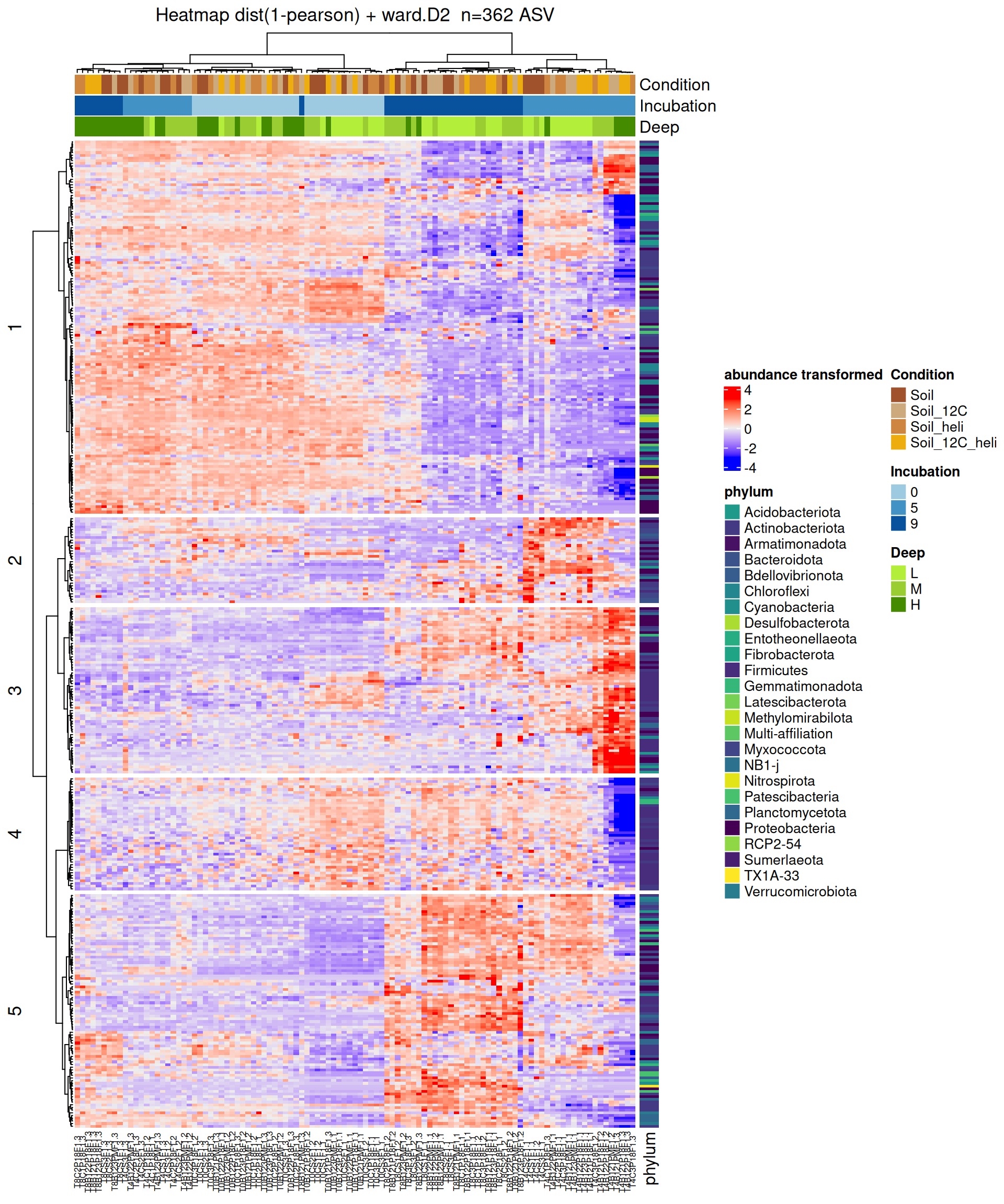
Heatmap based on Incubation contrasts
Heatmap
After the differential abundance analysis, a hierarchical clustering followed by a heatmap plot [5] were performed on DA ASV in at least one of the comparisons, with ComplexHeatmap R package.
Abundances matrix was transformed using vst function from DESeq2 R package to stabilize the variance and take into account for sequencing bias. Rows (=ASV) were centered and divided by the standard deviation.
Hierarchical clustering was performed for both rows and columns in two steps: 1/ calculate the pearson distance (1 - corr) and 2/ apply a clustering method with the Ward’s distance.
Code
#vector containing DAA ASV in at least one of contrastdaa_asv <- daa_deseq2_Incubation |>map_df(\(x) dplyr::select(x, ASV)) |>t() |>as.character() |>unique()
Code
# abundances were agglomerated by rank = Genus# calculate a variance stabilizing transformation VST# rows (= ASV) were centered and scaled vsd <- DESeq2::varianceStabilizingTransformation(dds, fitType="local", blind =FALSE)SummarizedExperiment::assay(vsd) <- SummarizedExperiment::assay(vsd)|>t() |>scale(center =TRUE, scale =TRUE) |>t()# select daa ASVvsd <- vsd[daa_asv,]#colData(vsd)#assay(vsd)#assay(vsd)["Cluster_xxx",]
The clustering revealed 5 groups of DA ASV between Incubation contrasts that share the same abundance profile. As explained by previous analyses, the profiles are mainly characterized by Incubation. The samples were not clustered by Condition. Then, within a group, profiles are interpreted on the basis of striking samples corresponding to combinations of interest in the 3 factors. Please note: the number of groups has been set arbitrarily on the basis of dendrogram visualization.
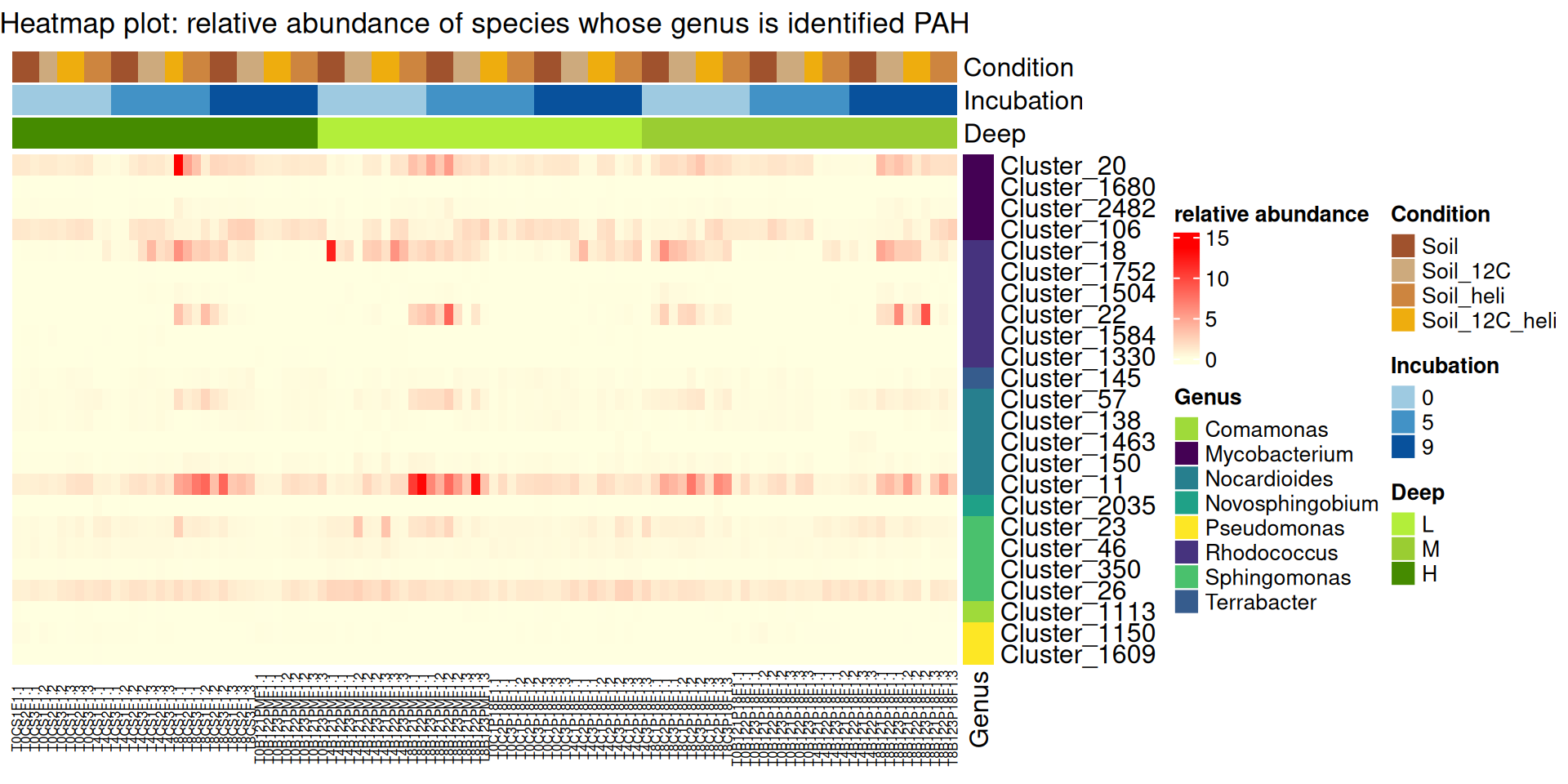
Few of species contain PAH-ring hydroxylating dioxygenases were identified in the soil samples. In fact, the taxonomic assignation is not enough sufficient, with some unknown species” and “Multi-affiliation” at the specie taxonomic rank. List of species included in the list of bacteria containing PAH-ring hydroxylating dioxygenases.
Code
# species in common between soil of samples and the list of bacteria containing PAH-ring hydroxylating dioxygenasesind <-tax_table(physeq_PAH_sp)[, "Species"] %in% listPAH$Specietax_table(physeq_PAH_sp)[ind, "Species"]
#subset taxa in PAH list: species within Genus of interestphyseq_PAH_sp <-subset_taxa(physeq_PAH_sp, Genus %in% listPAH$Genus)
So, we have considered genera provided from the list of bacteria that contain PAH-ring hydroxylating dioxygenases (file list_Species_PAH-ring.xlsx) to produce the heatmap plot.
The rows of heatmap plot correspond to the species identified in the soil samples and whose genus is included in the list of bacteria containing PAH-ring hydroxylating dioxygenases. This is the heatmap plot of the relative abundance of these species.
1. McMurdie PJ, Holmes S. Phyloseq: An r package for reproducible interactive analysis and graphics of microbiome census data. PloS one. 2013;8:e61217.
4. Benjamini Y, Hochberg Y. Controlling the false discovery rate: A practical and powerful approach to multiple testing. Journal of the Royal Statistical Society Series B (Methodological). 1995;57:289–300. http://www.jstor.org/stable/2346101.
5. Gu Z, Eils R, Schlesner M. Complex heatmaps reveal patterns and correlations in multidimensional genomic data. Bioinformatics. 2016;32:2847–9. doi:10.1093/bioinformatics/btw313.
Reuse
This document will not be accessible without prior agreement of the partners
A work by Migale Bioinformatics Facility
Université Paris-Saclay, INRAE, MaIAGE, 78350, Jouy-en-Josas, France
Université Paris-Saclay, INRAE, BioinfOmics, MIGALE bioinformatics facility, 78350, Jouy-en-Josas, France

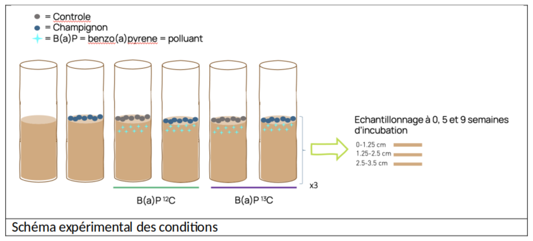 Soil microcosms in columns were carried out under 6 different conditions in triplicate.