metadata <- vroom::vroom("data/metadata.tsv") |>
  mutate(suspension = str_detect(treatment, "susp"),
         training   = str_detect(treatment, "tra"),
         animal     = str_extract(sample, "\\d+") |> as.numeric() %>%
           if_else(suspension, . + 10, .),
         animalID   = paste0(if_else(training, "T", "C"), animal) |>
           fct_relevel(paste0("C", 1:20), paste0("T", 1:20)),
         time       = if_else(suspension, "D21", "D0"),
         treatment  = fct_recode(treatment,
                                 "ctl D0" = "CTL", "train D0" = "tra", "ctl D21" = "susp", "train D21" = "tra+susp") |>
           fct_relevel("ctl D0", "train D0", "ctl D21", "train D21"),
         train      = if_else(training, "train", "ctl"),
         rowname = sample,
         .after = "sample"
         ) |>
  column_to_rownames()
metadata %>%
datatable()NEBULA
The aim of the study was to explore the impact of a specific preparation protocol prior to induction of microgravity on the composition of the intestinal microbiota
closed
collaboration
Note
This document is a report of the analyses performed. You will find all the code used to analyze these data. The version of the tools (maybe in code chunks) and their references are indicated, for questions of reproducibility.
Aim of the project
The aim of the study was to explore the impact of a specific preparation protocol prior to induction of microgravity on the composition of the intestinal microbiota.
Details are available here
Patners
- Olivier Rué - Migale bioinformatics facility - BioInfomics - INRAE
- Mahendra Mariadassou - Migale bioinformatics facility - BioInfomics - INRAE
- Bénédicte Goustard - DMEM - INRAE
- Christelle Ramonatxo - DMEM - INRAE
- Anthony Coste - DMEM - INRAE
Deliverables
Deliverables agreed at the preliminary meeting (Table 1).
| Definition | |
|---|---|
| 1 | HTML report |
Data management
Important
All data is managed by the migale facility for the duration of the project. Once the project is over, the Migale facility does not keep your data. We will provide you with the raw data and associated metadata that will be deposited on public repositories before the results are used. We can guide you in the submission process. We will then decide which files to keep, knowing that this report will also be provided to you and that the analyses can be replayed if needed.
Raw data
Here is the description of the samples:
Raw data were sent on November 20 and deposited on the front server and a copy was sent to the abaca server.
cd /home/orue/work/PROJECTS/NEBULA/
mkdir RAW_DATA
# Rename FASTQ files
for i in *_R1*.fastq.gz ; do id=$(echo $i |cut -d '_' -f 1 | cut -f 2 -d '-');cp $i RAW_DATA/${id}_R1.fastq.gz ; done
for i in *_R2*.fastq.gz ; do id=$(echo $i |cut -d '_' -f 1 | cut -f 2 -d '-');cp $i RAW_DATA/${id}_R2.fastq.gz ; done
scp -r RAW_DATA/ orue@abaca.maiage.inrae.fr:/backup/partage/migale/NEBULA/
Quality control
# seqkit
cd /home/orue/work/PROJECTS/NEBULA/
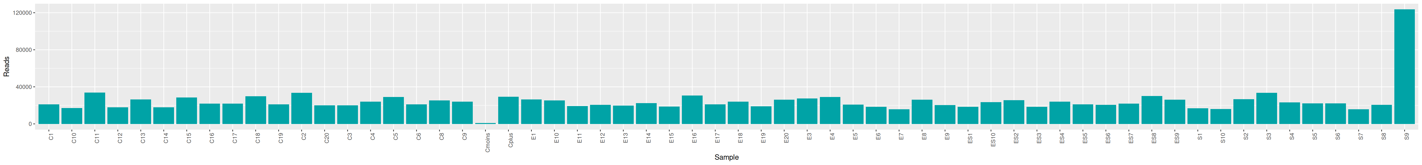
qsub -cwd -V -N seqkit -pe thread 4 -R y -b y "conda activate seqkit-2.0.0 && seqkit stats /home/orue/work/PROJECTS/NEBULA/RAW_DATA/*.fastq.gz -j 4 > raw_data.infos && conda deactivate"We can plot and display the number of reads to see if enough reads are present and if samples are homogeneous.
cd /home/orue/work/PROJECTS/NEBULA/
mkdir FASTQC LOGS
for i in /home/orue/work/PROJECTS/NEBULA/RAW_DATA/*.fastq.gz ; do echo "conda activate fastqc-0.11.9 && fastqc $i -o FASTQC && conda deactivate" >> fastqc.sh ; done
qarray -cwd -V -N fastqc -o LOGS -e LOGS fastqc.sh
qsub -cwd -V -N multiqc -o LOGS -e LOGS -b y "conda activate multiqc-1.11 && multiqc FASTQC -o MULTIQC && conda deactivate"
The MultiQC report shows expected metrics for Illumina Miseq sequencing data.
Bioinformatics
We used FROGS
Denoising
The first tool, called denoising.py allows to clean reads and product ASVs. Primers were removed, then sequences were denoised with DADA2
Warning
FROGS v5.0 (under development) was used.
export PATH="/home/orue/work/GIT/FROGS2023OK/libexec":$PATH
export PATH="/home/orue/work/GIT/FROGS2023OK/app":$PATH
export PYTHONPATH=`echo $(dirname $(dirname $(which preprocess.py)))/lib`:$PYTHONPATH
denoising.py illumina --merge-software pear --process dada2 --min-amplicon-size 250 --max-amplicon-size 580 --five-prim-primer GGGAGGCAGCAGTGGGGAATA --three-prim-primer GGATTAGATACCCTGGTA --R1-size 300 --R2-size 300 --nb-cpus 16 --pseudo-pooling --input-archive ../RAW_DATA/NEBULA.tar.gz --output-biom denoising.biom --output-fasta denoising.fasta --summary denoising.html --log-file denoising.log
The denoising report shows the amount of reads lost at each step and the length distribution of ASVs.
Note
~25% of the reads were removed because they don’t have the 5’ primer sequence. It happens sometimes and we cannot do anything.
Chimera removal
remove_chimera.py --input-fasta denoising.fasta --input-biom denoising.biom --nb-cpus 16 --summary remove_chimera.html --log remove_chimera.logThe chimera removel report shows that 8.3% of the sequences are detected as chimera.
Cluster filters
Now, we want to remove low-abundant clusters (abundance less the 0.005% of total abundance).
cluster_filters.py --input-fasta remove_chimera.fasta --input-biom remove_chimera_abundance.biom --nb-cpus 16 --log-file filters.log --output-biom filters.biom --summary filters.html --excluded filters_excluded.tsv --contaminant /db/outils/FROGS/contaminants/phi.fa --min-abundance 0.00005 --min-sample-presence 1 --output-fasta filters.fastaThe filters report shows how many clusters and sequences have been impacted by our filters. The 0.005% of total abundance corresponds to 44 sequences.
The filters have removed 87% of clusters, 620 ASVs are remaining, corresponding to 859,975 sequences (98.4% of sequences after chimera removal).
Taxonomic affiliation
We now performed a taxonomic assignation of ASVs with blast
taxonomic_affiliation.py --reference /db/outils/FROGS/assignation/silva_138.1_16S_pintail100/silva_138.1_16S_pintail100.fasta --input-biom filters.biom --input-fasta filters.fasta --output-biom affiliation.biom --summary affiliation.html --nb-cpus 16
affiliation_stats.py --input-biom affiliation.biom --output-file affiliations_stats.html --multiple-tag blast_affiliations --tax-consensus-tag blast_taxonomy --identity-tag perc_identity --coverage-tag perc_query_coverage
The affiliation report shows that all ASVs have been affiliated and a small part (10%) is multi-affiliated at Species level. The affiliation stats report shows that the coverage and identity metrics of blast hits are good.
Check affiliations with affiliationExplorer
When possible, I updated some affiliations to remove ambiguities.
Biostatistics
We now build a phyloseq object from the metadata file, the BIOM file and the tree file.
if(!file.exists("html/physeq.rds")){
  physeq <- import_frogs("data/cleaned.biom", taxMethod = "blast")
  sample_data(physeq) <- metadata
  phy_tree(physeq) <- read_tree("data/tree.nwk")
  ## remove negative and positive controls
  physeq <- subset_samples(physeq, !is.na(treatment)) %>%
    prune_taxa(taxa_sums(.) > 0, .)
  saveRDS(object = physeq, file="html/physeq.rds")
}else{
  physeq <- readRDS("html/physeq.rds")
}

physeq
phyloseq-class experiment-level object
otu_table() OTU Table: [ 609 taxa and 58 samples ]
sample_data() Sample Data: [ 58 samples by 12 sample variables ]
tax_table() Taxonomy Table: [ 609 taxa by 7 taxonomic ranks ]
phy_tree() Phylogenetic Tree: [ 609 tips and 608 internal nodes ]We also choose a custom palette and strip design
treat_pal <- set_names(x = c("#A6CEE3", "#B2DF8A", "#1F78B4", "#33A02C"),
                       nm = metadata$treatment |> levels())
train_pal <- c("FALSE" = "#A6CEE3", "TRUE" = "#B2DF8A")
train_pal2 <- c("ctl" = "#A6CEE3", "train" = "#B2DF8A")
train_pal_dark <- c("ctl" = "#1F78B4", "train" = "#33A02C")
treat_strip <- strip_nested(
  background_x = elem_list_rect(fill = c("grey80", "grey40", treat_pal)),
  text_x = elem_list_text(color = c(c("black", "white"), rep(c("black", "white"), each = 2)),
                          face = rep("bold", 6))
)
top_asv <- fantaxtic::top_taxa(physeq, n_taxa = 15000)
top_nested <- nested_top_taxa(physeq,
top_tax_level = "Phylum",
nested_tax_level = "Genus",
n_top_taxa = 10,
n_nested_taxa = 3)
p <- plot_nested_bar(ps_obj = top_nested$ps_obj,
top_level = "Phylum",
nested_level = "Genus") +
aes(x = animalID)
p + facet_nested(~ time + train, scales="free_x", space = "free_x",
strip = treat_strip) +
labs(x = "Animal") +
theme(legend.position = "bottom")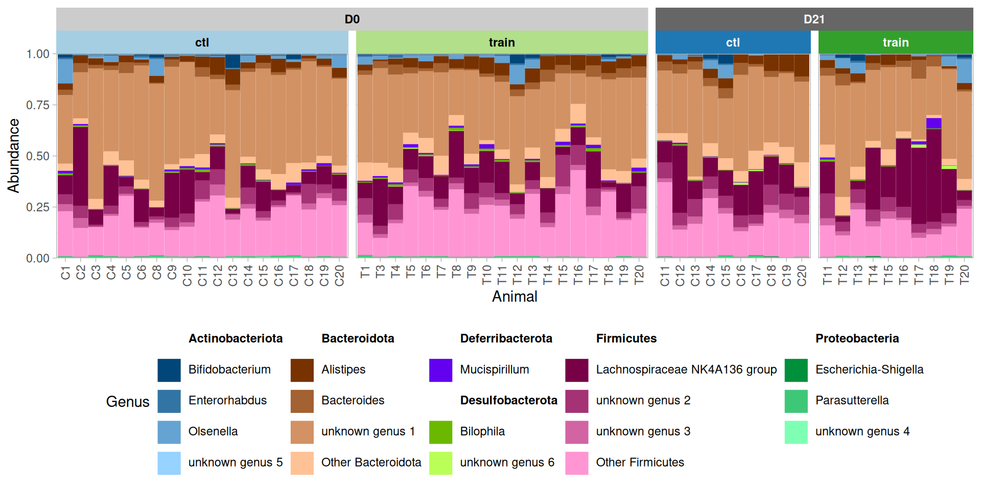
Alpha diversity analyses
We average diversity values obtained over 100 independant rarefactions and work with the average values.
## Diversity averaged over 100 different rarefactions
div_values <- map(1:100, \(i) rarefy_even_depth(physeq) |>  estimate_richness(measures = c("Observed", "Shannon")) |> rownames_to_column(var = "sample")) |>
  bind_rows(.id = "rep") |>
  summarise(across(c(Observed:Shannon), mean), .by = sample)
div_data <- inner_join(
  sample_data(physeq) |> as_tibble(),
  div_values,
  by = "sample"
) |>
pivot_longer(c(Observed, Shannon), names_to = "index", values_to = "diversity")The rarefaction curves show that the diversity is well captured across all conditions at 10,000 reads.
p <- ggrare(physeq, step = 500, color = "treatment", verbose = FALSE, se = FALSE, plot = FALSE)
p +
  geom_vline(xintercept = 10000, linetype = "dashed", color = "grey80") +
  scale_color_manual(values = treat_pal) +
  facet_nested(~ time + train, strip = treat_strip) +
  theme_bw() +
  theme(legend.position = "none")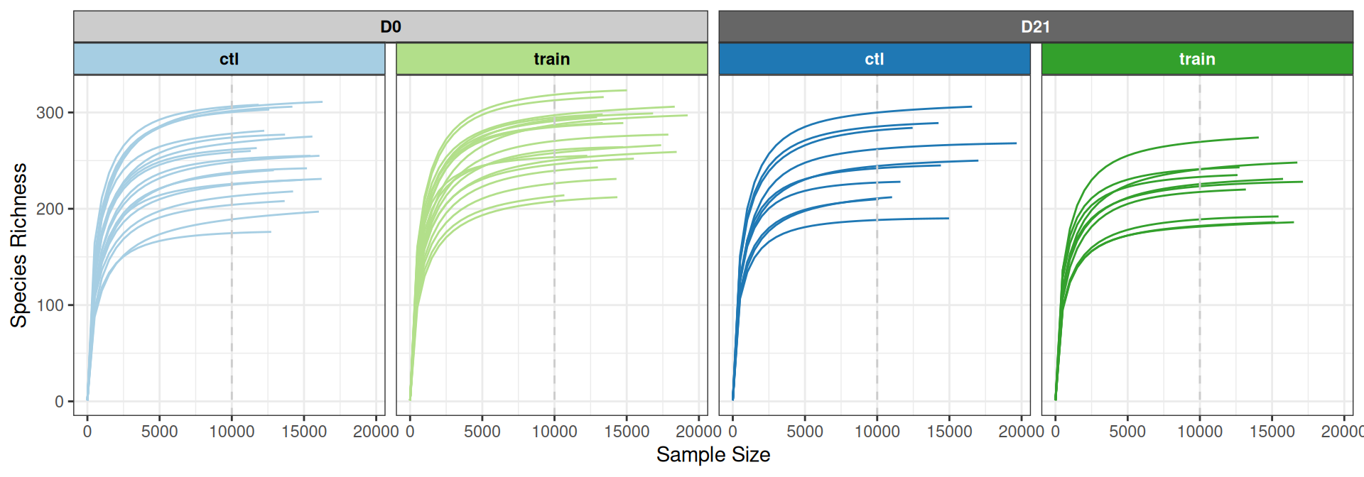
Let’s look in details at the Observed and Shannon diversity indexes. There seem to be small differences among treatments.
div_plot <- div_data |>
  ggplot(aes(x = treatment, y = diversity)) +
  geom_violin(aes(fill = treatment), alpha = 0.5) +
  geom_point(aes(colour = treatment),
             position = position_jitter(width = 0.15, height = 0)) +
  scale_colour_manual(values = treat_pal, aesthetics = c("colour", "fill")) +
  labs(x = "Treatment", y = "Diversity") +
  facet_wrap(~index, scales = "free_y") +
  theme_bw() +
  theme(legend.position = "none")
div_plot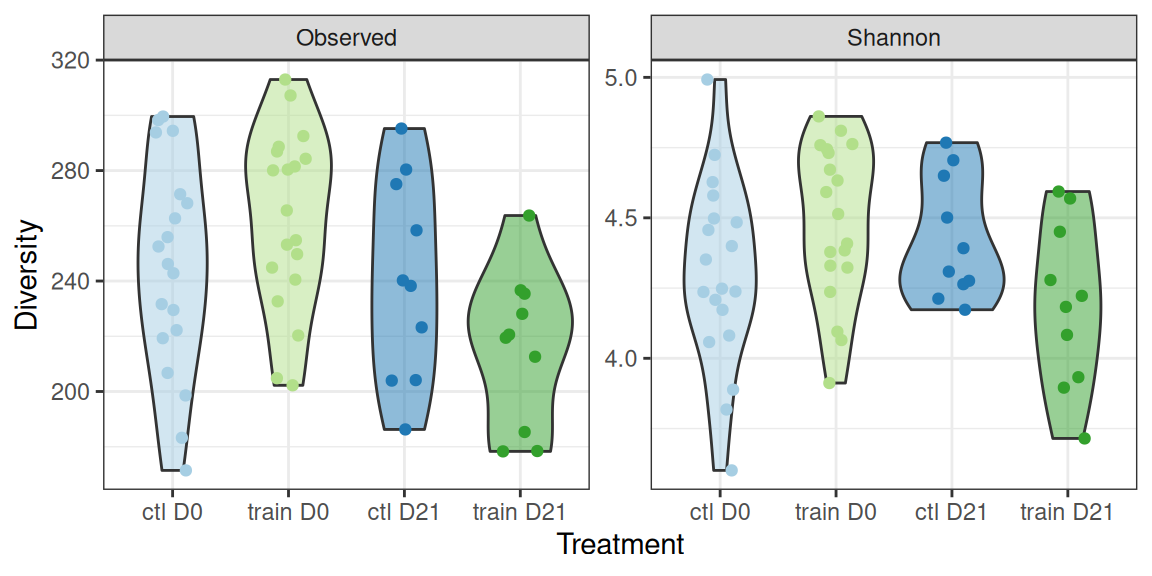
A Kruskal test (non-parametric one-way ANOVA) reveals significant differences between the treatments for both
- the observed richness
kruskal.test(diversity ~ treatment, data = div_data |> filter(index == "Observed"))
    Kruskal-Wallis rank sum test

data:  diversity by treatment
Kruskal-Wallis chi-squared = 10.168, df = 3, p-value = 0.01719- the shannon index
kruskal.test(diversity ~ treatment, data = div_data |> filter(index == "Shannon"))
    Kruskal-Wallis rank sum test

data:  diversity by treatment
Kruskal-Wallis chi-squared = 7.796, df = 3, p-value = 0.05042
A parametric one-way ANOVA reveals significant differences between the treatments for both
- the observed richness
aov(diversity ~ treatment, data = div_data |> filter(index == "Observed")) |>
  summary()
Df Sum Sq Mean Sq F value Pr(>F)
treatment 3 14353 4784 3.988 0.0123 *
Residuals 54 64787 1200
---
Signif. codes: 0 '***' 0.001 '**' 0.01 '*' 0.05 '.' 0.1 ' ' 1- the shannon index (only borderline significant in that case)
aov(diversity ~ treatment, data = div_data |> filter(index == "Shannon")) |>
  summary()
Df Sum Sq Mean Sq F value Pr(>F)
treatment 3 0.691 0.23040 2.719 0.0535 .
Residuals 54 4.576 0.08474
---
Signif. codes: 0 '***' 0.001 '**' 0.01 '*' 0.05 '.' 0.1 ' ' 1We can use the compact letter display (where groups with significantly different means don’t share a letter) to highlight differences between groups: - suspension appears to have no effect in the control group - suspension appears to decrease the diversity in the trained group - there are strong differences between the control and the trained group, which are highly mediated by the suspension (strong interaction effect).
div_plot +
  ## add cld display
  geom_text(data = . %>% create_cld_data(level = 0.05), aes(label = cld), vjust = 0)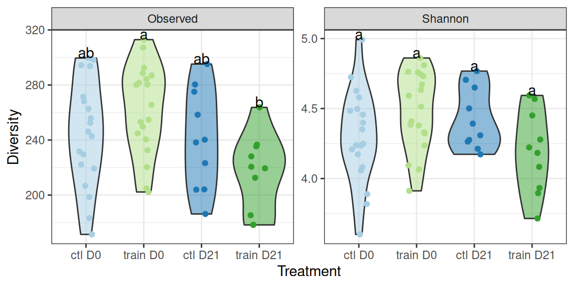
Warning
The previous results should be interpreted with caution as we didn’t account for the longitudinal effect: some mice are shared between ctl and ctl + susp on the one hand and train and train + susp on the other hand. The rest of the analyses focuses on specific comparisons to make sure there’s no such confouding factor.
In this section, we focus on the effet on training at time DO and compare the ctl and train groups. We don’t observe a significant effect of the group on the diversity (using a one-way ANOVA).
(div_plot %+% subset(div_data, time == "D0")) +
  geom_text(data = . %>% create_cld_data(level = 0.05), aes(label = cld), vjust = 0) +
  scale_x_discrete(name = "Training", labels = c("No training", "Training")) +
  NULL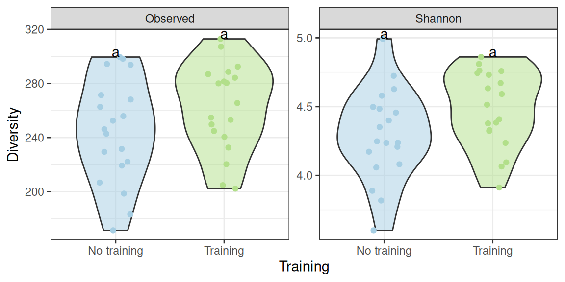
We can extract the exact p-values for the parametric test to confirm that the effect is not significant
## Observed diversity
aov(diversity ~ training, data = div_data |> filter(index == "Observed", time == "D0")) |> summary()
Df Sum Sq Mean Sq F value Pr(>F)
training 1 2947 2947 2.319 0.137
Residuals 36 45741 1271 ## Shannon diversity
aov(diversity ~ training, data = div_data |> filter(index == "Shannon", time == "D0")) |> summary() Df Sum Sq Mean Sq F value Pr(>F)
training 1 0.331 0.3311 3.528 0.0685 .
Residuals 36 3.379 0.0939
---
Signif. codes: 0 '***' 0.001 '**' 0.01 '*' 0.05 '.' 0.1 ' ' 1And likewise for the kruskall-wallis test (although in both cases, the effect is borderline significant for the Shannon diversity)
## Observed diversity
kruskal.test(diversity ~ training, data = div_data |> filter(index == "Observed", time == "D0"))
    Kruskal-Wallis rank sum test

data:  diversity by training
Kruskal-Wallis chi-squared = 1.6128, df = 1, p-value = 0.2041
## Shannon diversity
kruskal.test(diversity ~ training, data = div_data |> filter(index == "Shannon", time == "D0"))
    Kruskal-Wallis rank sum test

data:  diversity by training
Kruskal-Wallis chi-squared = 3.7692, df = 1, p-value = 0.0522We look at samples (untrained and trained)
p <- div_plot %+% subset(div_data, animal %in% 11:20)
p$layers[1:2] <- NULL
div_susp_plot <- p + geom_line(aes(group = animalID), linewidth = 0.8) +
  geom_point()
div_susp_plot + scale_color_manual(values = train_pal2) + aes(x = time, color = train) + labs(x = "Time")
We observe an significant (resp. borderline significant) decrease in the observed (resp. Shannon) alpha diversity using either a paired t-test
## Observed diversity
t.test(Pair(D0, D21) ~ 1, data = div_data_paired |> filter(index == "Observed"))
    Paired t-test

data:  Pair(D0, D21)
t = 3.8429, df = 19, p-value = 0.001097
alternative hypothesis: true mean difference is not equal to 0
95 percent confidence interval:
 14.51622 49.24278
sample estimates:
mean difference
        31.8795
## Shannon diversity
t.test(Pair(D0, D21) ~ 1, data = div_data_paired |> filter(index == "Shannon"))
    Paired t-test

data:  Pair(D0, D21)
t = 1.9631, df = 19, p-value = 0.06444
alternative hypothesis: true mean difference is not equal to 0
95 percent confidence interval:
 -0.009375002  0.292689478
sample estimates:
mean difference
      0.1416572
or its non parametric equivalent (Wilcoxon signed-rank test), for which both the observed and shannon diversities are significantly impacted by the suspension.
## Observed diversity
wilcox.test(Pair(D0, D21) ~ 1, data = div_data_paired |> filter(index == "Observed"))
    Wilcoxon signed rank exact test

data:  Pair(D0, D21)
V = 186, p-value = 0.001432
alternative hypothesis: true location shift is not equal to 0
## Shannon diversity
wilcox.test(Pair(D0, D21) ~ 1, data = div_data_paired |> filter(index == "Shannon"))
    Wilcoxon signed rank exact test

data:  Pair(D0, D21)
V = 163, p-value = 0.02958
alternative hypothesis: true location shift is not equal to 0
Warning
The observed decrease compounds both trained and untrained populations. Let’s look at both populations in turn to see if the same decrease is observed in both populations.
We don’t observe a clear-cut tendency in the alpha-diversity: overall suspension has no effect on (the diversity of) untrained mice.
p <- div_susp_plot %+% subset(div_data, animal %in% 11:20 & !training)
p + geom_line(aes(group = animalID, color = train)) +
  geom_point(aes(color = treatment)) +
  geom_text(data = . %>% create_cld_data(level = 0.05), aes(label = cld), vjust = 0) +
  scale_color_manual(values = treat_pal) + scale_x_discrete(labels = c("D0", "D21")) +
  labs(x = "Time")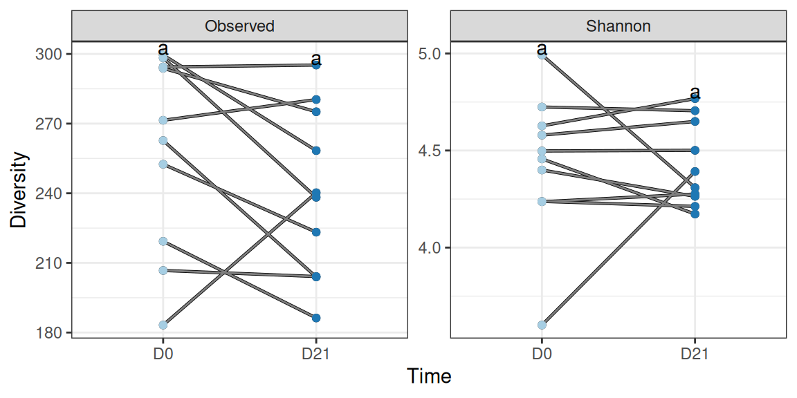
We can extract the exact p-values for the parametric test to confirm that the effect is not significant, even after pairing the samples.
## Observed diversity
t.test(Pair(D0, D21) ~ 1, data = div_data_paired |> filter(index == "Observed", !training))
    Paired t-test

data:  Pair(D0, D21)
t = 1.5814, df = 9, p-value = 0.1483
alternative hypothesis: true mean difference is not equal to 0
95 percent confidence interval:
 -7.614646 42.990646
sample estimates:
mean difference
         17.688
## Shannon diversity
t.test(Pair(D0, D21) ~ 1, data = div_data_paired |> filter(index == "Shannon", !training))
    Paired t-test

data:  Pair(D0, D21)
t = 0.088717, df = 9, p-value = 0.9312
alternative hypothesis: true mean difference is not equal to 0
95 percent confidence interval:
 -0.2528464  0.2734880
sample estimates:
mean difference
     0.01032081
And likewise for the Wilcoxon signed rank exact test.
## Observed diversity
wilcox.test(Pair(D0, D21) ~ 1, data = div_data_paired |> filter(index == "Observed", !training))
    Wilcoxon signed rank exact test

data:  Pair(D0, D21)
V = 43, p-value = 0.1309
alternative hypothesis: true location shift is not equal to 0
## Shannon diversity
wilcox.test(Pair(D0, D21) ~ 1, data = div_data_paired |> filter(index == "Shannon", !training))
    Wilcoxon signed rank exact test

data:  Pair(D0, D21)
V = 28, p-value = 1
alternative hypothesis: true location shift is not equal to 0
The results are markedly different among trained mice where a very strong effect of suspension on diversity is visible
p <- div_susp_plot %+% subset(div_data, animal %in% 11:20 & training)
p + geom_line(aes(group = animalID, color = train)) +
  geom_point(aes(color = treatment)) +
  geom_text(data = . %>% create_cld_data(level = 0.05), aes(label = cld), vjust = 0) +
  scale_color_manual(values = treat_pal) + scale_x_discrete(labels = c("D0", "D21")) +
  labs(x = "Time")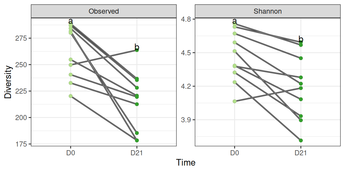
We can extract the exact p-values for the parametric test to confirm that the effect is very significant
## Observed diversity
t.test(Pair(D0, D21) ~ 1, data = div_data_paired |> filter(index == "Observed", training))
    Paired t-test

data:  Pair(D0, D21)
t = 4.1933, df = 9, p-value = 0.00233
alternative hypothesis: true mean difference is not equal to 0
95 percent confidence interval:
 21.21712 70.92488
sample estimates:
mean difference
         46.071
## Shannon diversity
t.test(Pair(D0, D21) ~ 1, data = div_data_paired |> filter(index == "Shannon", training))
    Paired t-test

data:  Pair(D0, D21)
t = 4.0171, df = 9, p-value = 0.003031
alternative hypothesis: true mean difference is not equal to 0
95 percent confidence interval:
 0.1192607 0.4267266
sample estimates:
mean difference
      0.2729937
And likewise for the Wilcoxon signed rank exact test
## Observed diversity
wilcox.test(Pair(D0, D21) ~ 1, data = div_data_paired |> filter(index == "Observed", training))
    Wilcoxon signed rank exact test

data:  Pair(D0, D21)
V = 54, p-value = 0.003906
alternative hypothesis: true location shift is not equal to 0
## Shannon diversity
wilcox.test(Pair(D0, D21) ~ 1, data = div_data_paired |> filter(index == "Shannon", training))
    Wilcoxon signed rank exact test

data:  Pair(D0, D21)
V = 53, p-value = 0.005859
alternative hypothesis: true location shift is not equal to 0
Warning
The previous results show that the effect of suspension depends on prior training, a typical evidence for a training:suspension interaction.
We now assess how the training affect the decrease induced by suspension. We do by taking advantage of the paired nature of the data and focus on the changes in diversity before doing a standard t-test on those difference.
div_data_paired |>
  ggplot(aes(x = training, y = D21 - D0)) +
  geom_violin(aes(fill = training), alpha = 0.5) + geom_point(aes(color = training)) +
  scale_color_manual(values = train_pal, aesthetics = c("color", "fill")) +
  facet_wrap(~index, scales = "free_y") +
  scale_x_discrete(labels = c("No training", "Training")) +
  labs(x = "Training", y = "Diversity change after suspension") +
  theme_bw() +
  theme(legend.position = "none") +
  NULL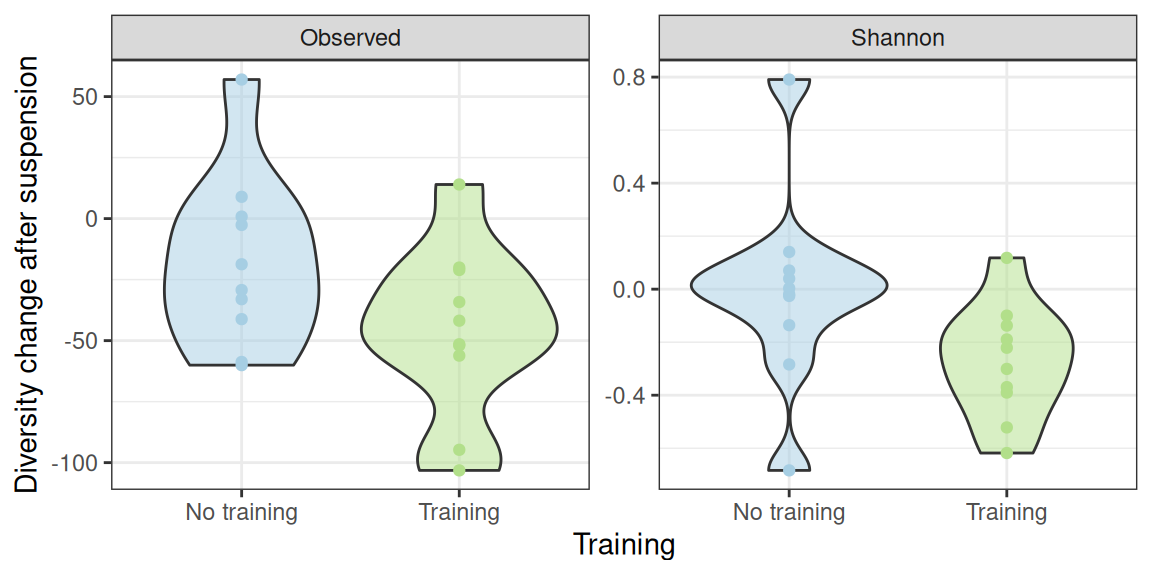
However the interaction is not significant (due to large intra-group variability) when using a t-test.
## Observed diversity
t.test(D21 - D0 ~ training, data = div_data_paired |> filter(index == "Observed"))
    Welch Two Sample t-test

data:  D21 - D0 by training
t = 1.8103, df = 17.994, p-value = 0.08698
alternative hypothesis: true difference in means between group FALSE and group TRUE is not equal to 0
95 percent confidence interval:
 -4.557256 61.323256
sample estimates:
mean in group FALSE  mean in group TRUE
            -17.688             -46.071
## Shannon diversity
t.test(D21 - D0 ~ training, data = div_data_paired |> filter(index == "Shannon"))
    Welch Two Sample t-test

data:  D21 - D0 by training
t = 1.9496, df = 14.502, p-value = 0.07083
alternative hypothesis: true difference in means between group FALSE and group TRUE is not equal to 0
95 percent confidence interval:
 -0.02535852  0.55070425
sample estimates:
mean in group FALSE  mean in group TRUE
        -0.01032081         -0.27299367
But becomes significant (for the Shannon index) when using a non-parametric kruskall-test.
## Observed diversity
kruskal.test(D21 - D0 ~ training, data = div_data_paired |> filter(index == "Observed"))
    Kruskal-Wallis rank sum test

data:  D21 - D0 by training
Kruskal-Wallis chi-squared = 2.2857, df = 1, p-value = 0.1306
## Shannon diversity
kruskal.test(D21 - D0 ~ training, data = div_data_paired |> filter(index == "Shannon"))
    Kruskal-Wallis rank sum test

data:  D21 - D0 by training
Kruskal-Wallis chi-squared = 4.48, df = 1, p-value = 0.03429
Warning
The lack of significance may be due to the one mouse in each group whose diversity increases drastically after suspension.
Beta diversity analyses
A global comparison (where lines connect to the two samples of a given mice, before after suspension) suggests for distances that
- smalls differences between
ctlandtrainbefore suspension (but with a high intra-group variability) - differences after suspension in both groups (effect along axis 1 for control samples, along axis 2 for trained samples)
For Bray-Curtis distances, we also observe that the effect of suspension on the microbiota is mediated by the training.
my_ord(physeq, dist_bc) +
  facet_grid(~training, labeller = labeller(training = c("TRUE" = "Training", "FALSE" = "No training"))) +
  theme(legend.position = "bottom")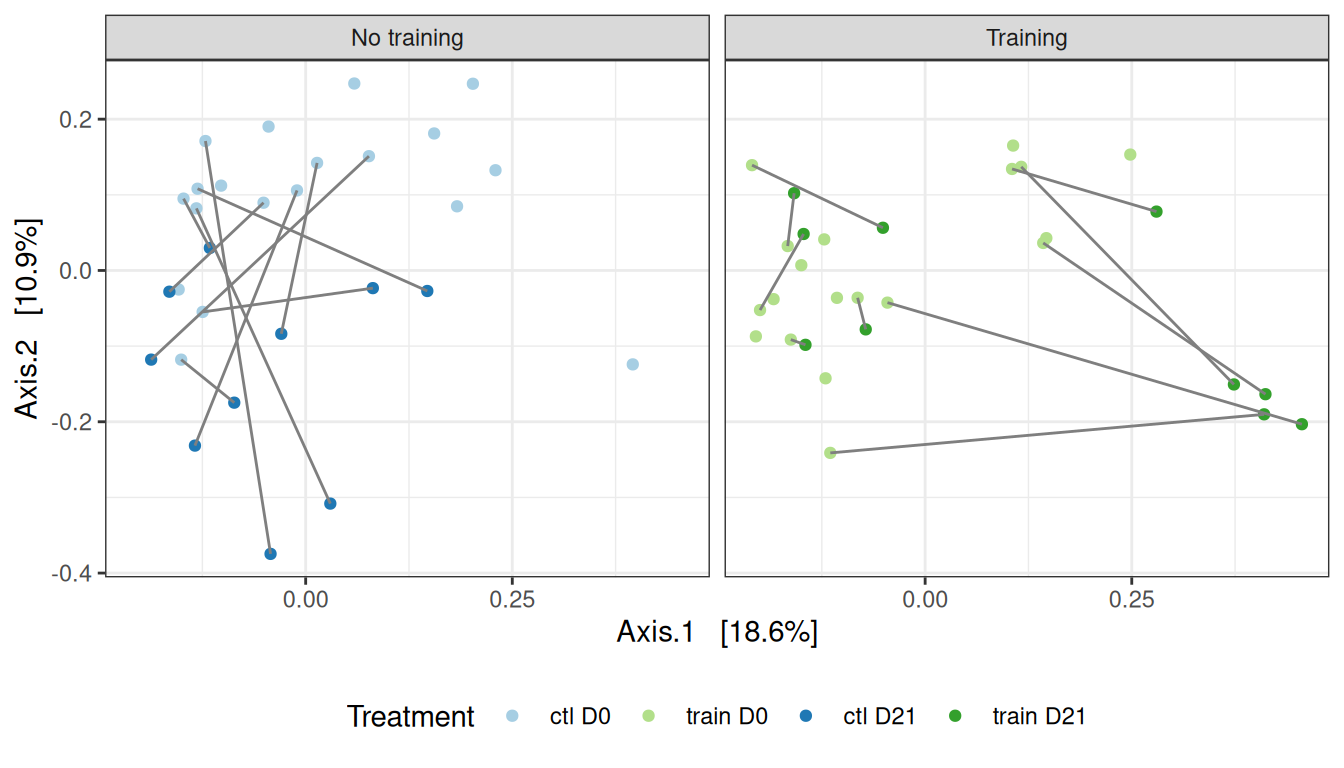
This can be confirmed using a PERMANOVA
## Global effect of treatment
vegan::adonis2(dist_bc ~ treatment, data = sample_data(physeq) |> as_tibble(), permutations = 999)
Permutation test for adonis under reduced model
Permutation: free
Number of permutations: 999
vegan::adonis2(formula = dist_bc ~ treatment, data = as_tibble(sample_data(physeq)), permutations = 999)
Df SumOfSqs R2 F Pr(>F)
Model 3 1.2199 0.12075 2.472 0.001 ***
Residual 54 8.8826 0.87925
Total 57 10.1024 1.00000
---
Signif. codes: 0 '***' 0.001 '**' 0.01 '*' 0.05 '.' 0.1 ' ' 1## Decomposition to assess the significance of the different effects
vegan::adonis2(dist_bc ~ training * suspension, data = sample_data(physeq) |> as_tibble(), permutations = 999)Permutation test for adonis under reduced model
Permutation: free
Number of permutations: 999
vegan::adonis2(formula = dist_bc ~ training * suspension, data = as_tibble(sample_data(physeq)), permutations = 999)
Df SumOfSqs R2 F Pr(>F)
Model 3 1.2199 0.12075 2.472 0.001 ***
Residual 54 8.8826 0.87925
Total 57 10.1024 1.00000
---
Signif. codes: 0 '***' 0.001 '**' 0.01 '*' 0.05 '.' 0.1 ' ' 1For UniFrac distances, the perturbations seems to impact both trained and control mice similarly.
my_ord(physeq, dist_uf) +
  facet_grid(~training, labeller = labeller(training = c("TRUE" = "Training", "FALSE" = "No training"))) +
  theme(legend.position = "bottom")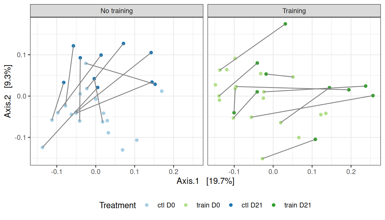
This can be confirmed using a PERMANOVA
## Global effect of treatment
vegan::adonis2(dist_uf ~ treatment, data = sample_data(physeq) |> as_tibble(), permutations = 999)
Permutation test for adonis under reduced model
Permutation: free
Number of permutations: 999
vegan::adonis2(formula = dist_uf ~ treatment, data = as_tibble(sample_data(physeq)), permutations = 999)
Df SumOfSqs R2 F Pr(>F)
Model 3 0.32258 0.11028 2.2311 0.001 ***
Residual 54 2.60250 0.88972
Total 57 2.92508 1.00000
---
Signif. codes: 0 '***' 0.001 '**' 0.01 '*' 0.05 '.' 0.1 ' ' 1## Decomposition to assess the significance of the different effects
vegan::adonis2(dist_uf ~ training * suspension, data = sample_data(physeq) |> as_tibble(), permutations = 999)Permutation test for adonis under reduced model
Permutation: free
Number of permutations: 999
vegan::adonis2(formula = dist_uf ~ training * suspension, data = as_tibble(sample_data(physeq)), permutations = 999)
Df SumOfSqs R2 F Pr(>F)
Model 3 0.32258 0.11028 2.2311 0.001 ***
Residual 54 2.60250 0.88972
Total 57 2.92508 1.00000
---
Signif. codes: 0 '***' 0.001 '**' 0.01 '*' 0.05 '.' 0.1 ' ' 1We now focus on the effect of training before suspension and don’t observe much differences at the community level.
The distance between the group is statistically significant but very small.
my_ord(subset_samples(physeq, time == "D0"), dist_bc) +
  stat_ellipse() +
  annotate(x = 0, y = -0.34, geom = "text", label= "Training", color = train_pal2["train"], fontface = "bold") +
  annotate(x = 0, y = 0.28, geom = "text", label= "No training", color = train_pal2["ctl"], fontface = "bold") +
  theme(legend.position = "none")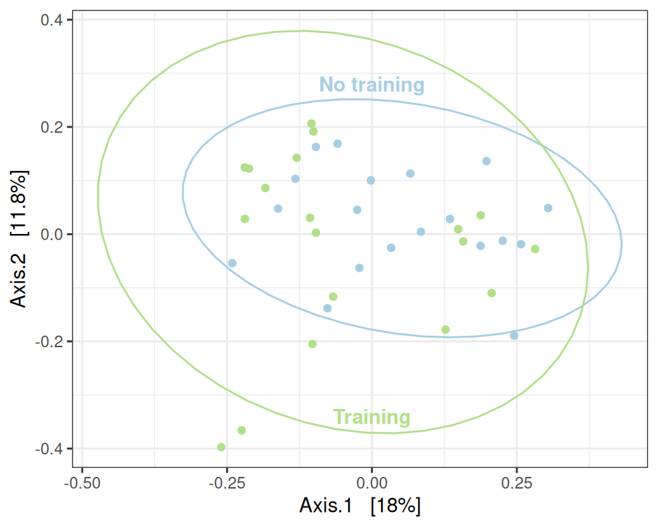
# theme(legend.position = c(1, 1), legend.justification = c(1, 1), legend.background = element_rect(fill = NA))This can be confirmed using a PERMANOVA (valid since the result of betadisper is not significant).
## Global effect of treatment
my_adonis(subset_samples(physeq, time == "D0"), dist_bc, "treatment")
Betadisper test
Analysis of Variance Table
Response: Distances
Df Sum Sq Mean Sq F value Pr(>F)
Groups 1 0.009959 0.0099591 1.507 0.2276
Residuals 36 0.237906 0.0066085
PERMANOVA test
Permutation test for adonis under reduced model
Permutation: free
Number of permutations: 999
vegan::adonis2(formula = as.formula(glue::glue("subdist ~ {group}")), data = as_tibble(sample_data(physeq)), permutations = permutations)
Df SumOfSqs R2 F Pr(>F)
Model 1 0.2664 0.04423 1.6659 0.031 *
Residual 36 5.7561 0.95577
Total 37 6.0225 1.00000
---
Signif. codes: 0 '***' 0.001 '**' 0.01 '*' 0.05 '.' 0.1 ' ' 1The distance between the groups is not significant.
my_ord(subset_samples(physeq, time == "D0"), dist_uf) +
  stat_ellipse() +
  annotate(x = -0.19, y = -0.15, geom = "text", label= "Training", color = train_pal2["train"], fontface = "bold") +
  annotate(x = 0, y = 0.2, geom = "text", label= "No training", color = train_pal2["ctl"], fontface = "bold") +
  theme(legend.position = "none")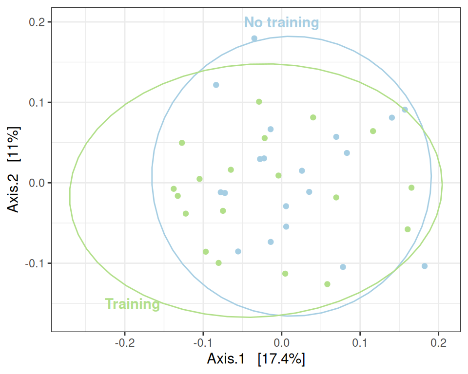
# theme(legend.position = c(1, 1), legend.justification = c(1, 1), legend.background = element_rect(fill = NA))This can be confirmed using a PERMANOVA (valid since the result of betadisper is not significant).
## Global effect of treatment
my_adonis(subset_samples(physeq, time == "D0"), dist_uf, "treatment")
Betadisper test
Analysis of Variance Table
Response: Distances
Df Sum Sq Mean Sq F value Pr(>F)
Groups 1 0.000035 0.00003524 0.0377 0.8471
Residuals 36 0.033645 0.00093459
PERMANOVA test
Permutation test for adonis under reduced model
Permutation: free
Number of permutations: 999
vegan::adonis2(formula = as.formula(glue::glue("subdist ~ {group}")), data = as_tibble(sample_data(physeq)), permutations = permutations)
Df SumOfSqs R2 F Pr(>F)
Model 1 0.0526 0.03018 1.1203 0.283
Residual 36 1.6904 0.96982
Total 37 1.7429 1.00000 We now assess the effect of suspension on trained and control mice independently. We consider 3 approaches:
- global analyses on the 20 mice that were submitted to suspension (to preserve a balanced design), using strata (to preserve the longitudinal structure).
- analyses of the effect of suspension for each population independently
- analyses of the changes in composition (quantified by beta-diversity)
Global analysis
my_ord(subset_samples(physeq, animal %in% 11:20), dist_bc) +
  stat_ellipse() +
  facet_grid(~training, labeller = labeller(training = c("FALSE" = "No training", "TRUE" = "Training"))) +
  geom_text(data = tibble(
    x = c(-0.27, -0.32, -0.25, 0.25),
    y = c(0.2, -0.3, 0.2, -0.24),
    label = c("D0", "D21", "D0", "D21"),
    training = c(FALSE, FALSE, TRUE, TRUE),
    treatment = c("ctl D0", "ctl D21", "train D0", "train D21")
  ),
  aes(x = x, y = y, label= label), fontface = "bold") +
  theme(legend.position = "none")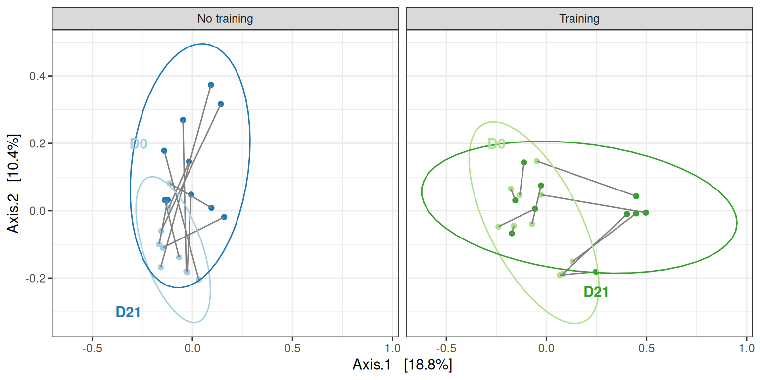
# theme(legend.position = c(1, 1), legend.justification = c(1, 1), legend.background = element_rect(fill = NA))We confirm the effect of treatment on this smaller dataset, using appropriate permutation scheme that preserve the design of the dataset.
permutations <- with(
  subset_samples(physeq, animal %in% 11:20) |> sample_data() |> as_tibble(),
  permute::how(within = permute::Within(type = "free"), plots = permute::Plots(strata = animalID, type = "free"),
               nperm = 999)
)
my_adonis(subset_samples(physeq, animal %in% 11:20), dist_bc, "treatment", permutations = permutations)
Betadisper test
Analysis of Variance Table
Response: Distances
Df Sum Sq Mean Sq F value Pr(>F)
Groups 3 0.007128 0.0023760 0.5168 0.6734
Residuals 36 0.165522 0.0045978
PERMANOVA test
Permutation test for adonis under reduced model
Plots: animalID, plot permutation: free
Permutation: free
Number of permutations: 999
vegan::adonis2(formula = as.formula(glue::glue("subdist ~ {group}")), data = as_tibble(sample_data(physeq)), permutations = permutations)
Df SumOfSqs R2 F Pr(>F)
Model 3 1.1410 0.15676 2.2309 0.001 ***
Residual 36 6.1375 0.84324
Total 39 7.2785 1.00000
---
Signif. codes: 0 '***' 0.001 '**' 0.01 '*' 0.05 '.' 0.1 ' ' 1Control mice
my_ord(subset_samples(physeq, animal %in% 11:20 & !training), dist_bc) +
  stat_ellipse() +
  geom_text(data = tibble(
    x = c(0.2, -0.32, -0.25, 0.25),
    y = c(-0.27, -0.27, 0.2, -0.24),
    label = c("D0", "D21", "D0", "D21"),
    training = c(FALSE, FALSE, TRUE, TRUE),
    treatment = c("ctl D0", "ctl D21", "train D0", "train D21")
  ) |> filter(!training),
  aes(x = x, y = y, label= label), fontface = "bold") +
theme(legend.position = "none") 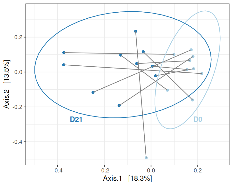
# theme(legend.position = c(0, 0), legend.justification = c(0, 0), legend.background = element_rect(fill = NA))my_adonis(subset_samples(physeq, animal %in% 11:20 & !training), dist_bc, "suspension", permutations = 999)Betadisper test
Analysis of Variance Table
Response: Distances
Df Sum Sq Mean Sq F value Pr(>F)
Groups 1 0.003986 0.0039863 0.8576 0.3667
Residuals 18 0.083665 0.0046480
PERMANOVA test
Permutation test for adonis under reduced model
Permutation: free
Number of permutations: 999
vegan::adonis2(formula = as.formula(glue::glue("subdist ~ {group}")), data = as_tibble(sample_data(physeq)), permutations = permutations)
Df SumOfSqs R2 F Pr(>F)
Model 1 0.4853 0.14191 2.9769 0.001 ***
Residual 18 2.9342 0.85809
Total 19 3.4195 1.00000
---
Signif. codes: 0 '***' 0.001 '**' 0.01 '*' 0.05 '.' 0.1 ' ' 1Trained mice
my_ord(subset_samples(physeq, animal %in% 11:20 & training), dist_bc) +
  geom_text(data = ~ . |> filter(training, suspension),
            aes(label = animalID), hjust = 0) +
  stat_ellipse() +
  geom_text(data = tibble(
    x = c(0.2, -0.32, -0.45, 0.25),
    y = c(-0.27, -0.27, 0.2, -0.26),
    label = c("D0", "D21", "D0", "D21"),
    training = c(FALSE, FALSE, TRUE, TRUE),
    treatment = c("ctl D0", "ctl D21", "train D0", "train D21")
  ) |> filter(training),
  aes(x = x, y = y, label= label), fontface = "bold") +
theme(legend.position = "none") 
  # theme(legend.position = c(0, 0), legend.justification = c(0, 0), legend.background = element_rect(fill = NA))
# theme(legend.position = c(1, 1), legend.justification = c(1, 1), legend.background = element_rect(fill = NA))my_adonis(subset_samples(physeq, animal %in% 11:20 & training), dist_bc, "suspension", permutations = 999)Betadisper test
Analysis of Variance Table
Response: Distances
Df Sum Sq Mean Sq F value Pr(>F)
Groups 1 0.000000 0.0000004 1e-04 0.9928
Residuals 18 0.081905 0.0045503
PERMANOVA test
Permutation test for adonis under reduced model
Permutation: free
Number of permutations: 999
vegan::adonis2(formula = as.formula(glue::glue("subdist ~ {group}")), data = as_tibble(sample_data(physeq)), permutations = permutations)
Df SumOfSqs R2 F Pr(>F)
Model 1 0.4184 0.11553 2.3512 0.026 *
Residual 18 3.2033 0.88447
Total 19 3.6217 1.00000
---
Signif. codes: 0 '***' 0.001 '**' 0.01 '*' 0.05 '.' 0.1 ' ' 1Effect size
effect_size_data <- extract_effect_size(physeq, dist_bc)
ggplot(effect_size_data, aes(x = training, y = distance)) +
  geom_violin(aes(fill = treatment), alpha = 0.5) + geom_point(aes(color = treatment)) +
  scale_color_manual(values = treat_pal, aesthetics = c("color", "fill")) +
  scale_x_discrete(name = "Training", labels = c("No training", "Training")) +
  labs(y = "Effect of suspension\nDistance between D0 and D21") +
  theme_bw() +
  theme(legend.position = "none")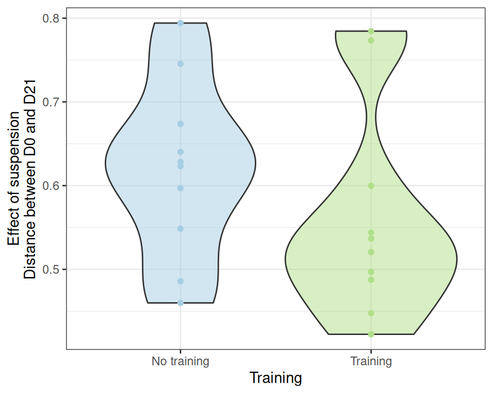
Unfortunately, we can’t significantly conclude that the effect of suspension is stronger in control samples than in trained samples using a t-test (probably because of the high variability)
t.test(distance ~ training, data = effect_size_data)
    Welch Two Sample t-test

data:  distance by training
t = 1.1305, df = 17.465, p-value = 0.2736
alternative hypothesis: true difference in means between group FALSE and group TRUE is not equal to 0
95 percent confidence interval:
 -0.05029667  0.16691873
sample estimates:
mean in group FALSE  mean in group TRUE
          0.6196725           0.5613614
nor a Kruskal test
kruskal.test(distance ~ training, data = effect_size_data)
    Kruskal-Wallis rank sum test

data:  distance by training
Kruskal-Wallis chi-squared = 1.8514, df = 1, p-value = 0.1736
However, if we find that two of the trained mice have a very strong response to suspension. Those mice are T16 and T18.
effect_size_data |> filter(training, distance >= 0.650)# A tibble: 2 × 13
Sample_1 distance suspension training animal animalID time train treatment
<chr> <dbl> <lgl> <lgl> <dbl> <fct> <chr> <chr> <fct>
1 E16 0.785 FALSE TRUE 16 T16 D0 train train D0
2 E18 0.773 FALSE TRUE 18 T18 D0 train train D0
# ℹ 4 more variables: MAV <dbl>, DeltaMAV <dbl>, Force <dbl>, DeltaForce <dbl>If we remove them before repeating the analyses, we reach different conclusions
ggplot(effect_size_data |> filter(!(training & distance >= 0.650)), aes(x = training, y = distance)) +
  geom_violin(aes(fill = treatment), alpha = 0.5) + geom_point(aes(color = treatment)) +
  scale_color_manual(values = treat_pal, aesthetics = c("color", "fill")) +
  scale_x_discrete(name = "Training", labels = c("No training", "Training")) +
  labs(y = "Effect of suspension\nDistance between D0 and D21") +
  theme_bw() +
  theme(legend.position = "none")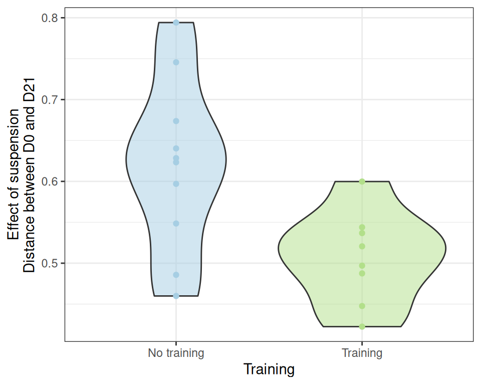
with both the standard t-test
t.test(distance ~ training, data = effect_size_data |> filter(!(training & distance >= 0.650)))
    Welch Two Sample t-test

data:  distance by training
t = 2.9162, df = 14.281, p-value = 0.01109
alternative hypothesis: true difference in means between group FALSE and group TRUE is not equal to 0
95 percent confidence interval:
 0.02996937 0.19547064
sample estimates:
mean in group FALSE  mean in group TRUE
          0.6196725           0.5069525
and a Kruskal test
kruskal.test(distance ~ training, data = effect_size_data |> filter(!(training & distance >= 0.650)))
    Kruskal-Wallis rank sum test

data:  distance by training
Kruskal-Wallis chi-squared = 5.3368, df = 1, p-value = 0.02088
showing that the lack of significance arises from these two animals reacting quite differently than the other trained mice.
Global analysis
my_ord(subset_samples(physeq, animal %in% 11:20), dist_uf) +
  stat_ellipse() +
  geom_text(data = tibble(
    x = c(0.22, -0.32, -0.025, -0.35),
    y = c(0.05, 0, 0.21, 0.15),
    label = c("D0", "D21", "D0", "D21"),
    training = c(FALSE, FALSE, TRUE, TRUE),
    treatment = c("ctl D0", "ctl D21", "train D0", "train D21")
  ),
  aes(x = x, y = y, label= label), fontface = "bold") +
  facet_grid(~training, labeller = labeller(training = c("FALSE" = "No training", "TRUE" = "Training"))) +
theme(legend.position = "none") 
# theme(legend.position = c(0, 1), legend.justification = c(0, 1), legend.background = element_rect(fill = NA))We confirm the effect of treatment on this smaller dataset, using appropriate permutation scheme that preserve the design of the dataset.
permutations <- with(
  subset_samples(physeq, animal %in% 11:20) |> sample_data() |> as_tibble(),
  permute::how(within = permute::Within(type = "free"), plots = permute::Plots(strata = animalID, type = "free"),
               nperm = 999)
)
my_adonis(subset_samples(physeq, animal %in% 11:20), dist_uf, "treatment", permutations = permutations)
Betadisper test
Analysis of Variance Table
Response: Distances
Df Sum Sq Mean Sq F value Pr(>F)
Groups 3 0.001142 0.00038069 0.2943 0.8293
Residuals 36 0.046575 0.00129374
PERMANOVA test
Permutation test for adonis under reduced model
Plots: animalID, plot permutation: free
Permutation: free
Number of permutations: 999
vegan::adonis2(formula = as.formula(glue::glue("subdist ~ {group}")), data = as_tibble(sample_data(physeq)), permutations = permutations)
Df SumOfSqs R2 F Pr(>F)
Model 3 0.34021 0.16281 2.3337 0.001 ***
Residual 36 1.74938 0.83719
Total 39 2.08959 1.00000
---
Signif. codes: 0 '***' 0.001 '**' 0.01 '*' 0.05 '.' 0.1 ' ' 1Control mice
my_ord(subset_samples(physeq, animal %in% 11:20 & !training), dist_uf) +
  stat_ellipse() +
  geom_text(data = tibble(
    x = c(-0.2, 0.25, -0.25, 0.25),
    y = c(0, 0, 0.2, -0.24),
    label = c("D0", "D21", "D0", "D21"),
    training = c(FALSE, FALSE, TRUE, TRUE),
    treatment = c("ctl D0", "ctl D21", "train D0", "train D21")
  ) |> filter(!training),
  aes(x = x, y = y, label= label), fontface = "bold") +
theme(legend.position = "none") 
  # theme(legend.position = c(0, 0), legend.justification = c(0, 0), legend.background = element_rect(fill = NA))
# theme(legend.position = c(0, 0), legend.justification = c(0, 0), legend.background = element_rect(fill = NA))my_adonis(subset_samples(physeq, animal %in% 11:20 & !training), dist_uf, "suspension", permutations = 999)Betadisper test
Analysis of Variance Table
Response: Distances
Df Sum Sq Mean Sq F value Pr(>F)
Groups 1 0.000217 0.00021706 0.1219 0.731
Residuals 18 0.032038 0.00177990
PERMANOVA test
Permutation test for adonis under reduced model
Permutation: free
Number of permutations: 999
vegan::adonis2(formula = as.formula(glue::glue("subdist ~ {group}")), data = as_tibble(sample_data(physeq)), permutations = permutations)
Df SumOfSqs R2 F Pr(>F)
Model 1 0.14828 0.14511 3.0552 0.001 ***
Residual 18 0.87359 0.85489
Total 19 1.02187 1.00000
---
Signif. codes: 0 '***' 0.001 '**' 0.01 '*' 0.05 '.' 0.1 ' ' 1Trained mice
my_ord(subset_samples(physeq, animal %in% 11:20 & training), dist_uf) +
  stat_ellipse() +
  geom_text(data = tibble(
    x = c(0.2, -0.32, -0.08, 0.4),
    y = c(-0.27, -0.27, 0.21, -0),
    label = c("D0", "D21", "D0", "D21"),
    training = c(FALSE, FALSE, TRUE, TRUE),
    treatment = c("ctl D0", "ctl D21", "train D0", "train D21")
  ) |> filter(training),
  aes(x = x, y = y, label= label), fontface = "bold") +
theme(legend.position = "none") 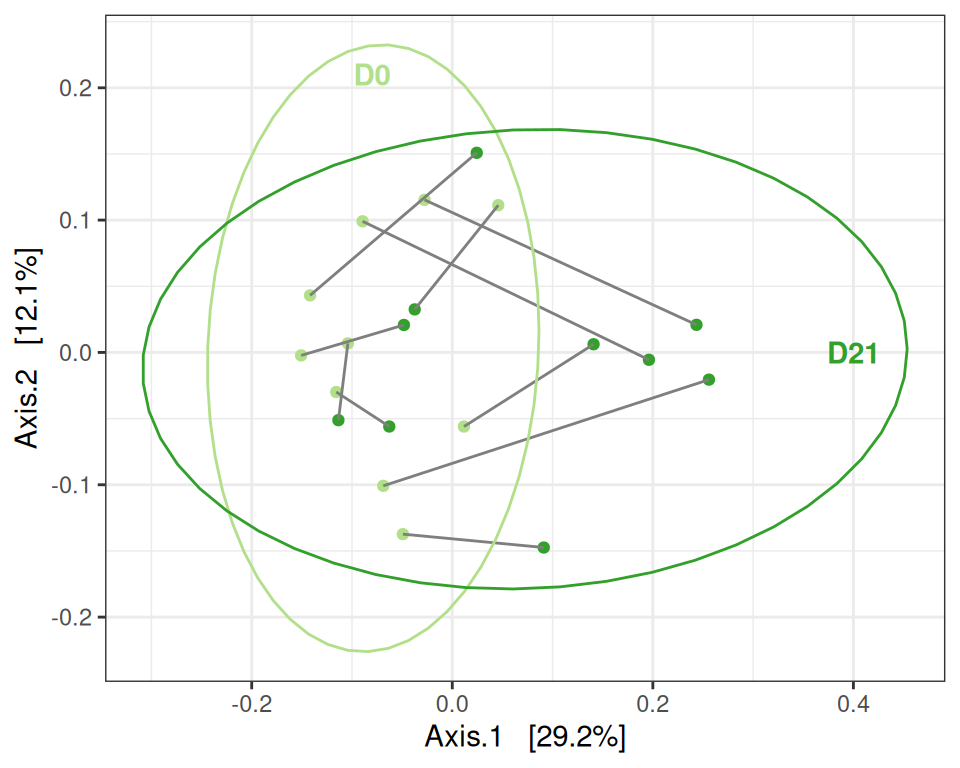
  # theme(legend.position = c(0, 0), legend.justification = c(0, 0), legend.background = element_rect(fill = NA))
# theme(legend.position = c(1, 1), legend.justification = c(1, 1), legend.background = element_rect(fill = NA))my_adonis(subset_samples(physeq, animal %in% 11:20 & training), dist_uf, "suspension", permutations = 999)Betadisper test
Analysis of Variance Table
Response: Distances
Df Sum Sq Mean Sq F value Pr(>F)
Groups 1 0.0008908 0.00089084 1.1028 0.3075
Residuals 18 0.0145397 0.00080776
PERMANOVA test
Permutation test for adonis under reduced model
Permutation: free
Number of permutations: 999
vegan::adonis2(formula = as.formula(glue::glue("subdist ~ {group}")), data = as_tibble(sample_data(physeq)), permutations = permutations)
Df SumOfSqs R2 F Pr(>F)
Model 1 0.14403 0.14123 2.9602 0.004 **
Residual 18 0.87580 0.85877
Total 19 1.01983 1.00000
---
Signif. codes: 0 '***' 0.001 '**' 0.01 '*' 0.05 '.' 0.1 ' ' 1Effect size
effect_size_data <- extract_effect_size(physeq, dist_uf)
ggplot(effect_size_data, aes(x = training, y = distance)) +
  geom_violin(aes(fill = treatment), alpha = 0.5) + geom_point(aes(color = treatment)) +
  scale_color_manual(values = treat_pal, aesthetics = c("color", "fill")) +
  scale_x_discrete(name = "Training", labels = c("No training", "Training")) +
  labs(y = "Effect of suspension\nDistance between D0 and D21") +
  theme_bw() +
  theme(legend.position = "none")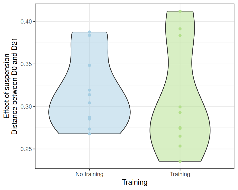
Unfortunately, we can’t significantly conclude that the effect of suspension is stronger in control samples than in trained samples using a t-test (probably because of the high variability)
t.test(distance ~ training, data = effect_size_data)
    Welch Two Sample t-test

data:  distance by training
t = 0.36246, df = 15.888, p-value = 0.7218
alternative hypothesis: true difference in means between group FALSE and group TRUE is not equal to 0
95 percent confidence interval:
 -0.04261936  0.06018689
sample estimates:
mean in group FALSE  mean in group TRUE
          0.3170762           0.3082925
nor a Kruskal test
kruskal.test(distance ~ training, data = effect_size_data)
    Kruskal-Wallis rank sum test

data:  distance by training
Kruskal-Wallis chi-squared = 0.57143, df = 1, p-value = 0.4497
Differential abundances
The search for biormarkers gives a lot less interesting results…
We perform a Linear Discriminant Analysis (LDA) to find whether the microbiota is predictive of the treatment. We find a few ASV (but not that many) which are predictive of the treatment.
physeq_mpse <- physeq |> rarefy_even_depth(rngseed = 20240228) |> as.MPSE()
physeq_diff <- physeq_mpse
physeq_diff %<>%
  mp_cal_abundance( # for each samples
    .abundance = RareAbundance
  ) %>%
  mp_cal_abundance( # for each samples
    .abundance = RareAbundance,
    .group = treatment
  ) %>%
  ## Add discriminant analysis
  mp_diff_analysis(
    .abundance = RareAbundance,
    .group = treatment,
    first.test.alpha = 0.1
  )
p <- physeq_diff %>%
mp_plot_diff_boxplot(
.group = treatment,
) %>%
set_diff_boxplot_color(
values = treat_pal,
guide = guide_legend(title=NULL, reverse = TRUE)
)
p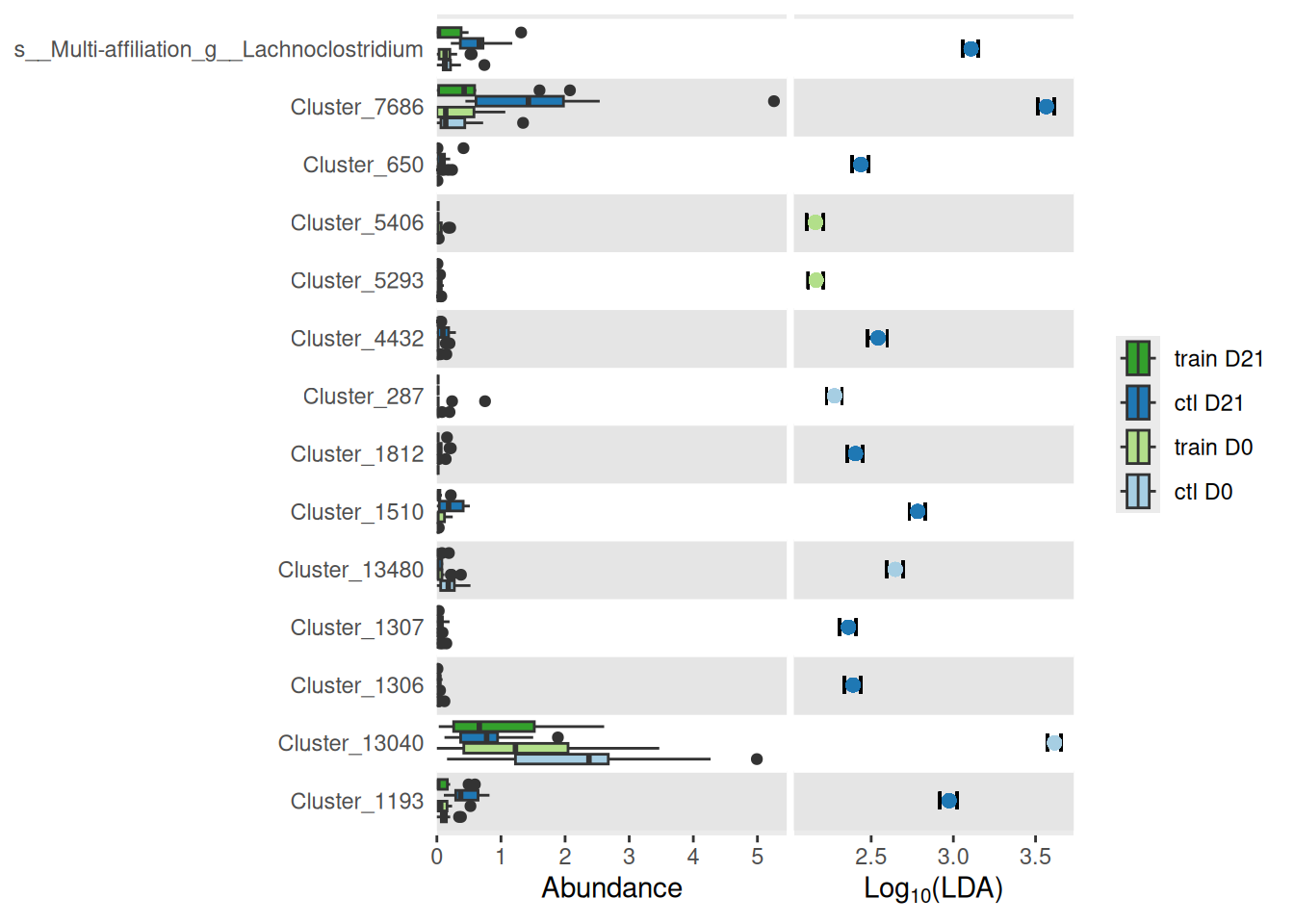
Using a different version of LEFSe (on clr-transformed data), we find quite different results. Overall, the results are
lefse_results <- lefse(physeq, group = "treatment", padj.threshold = 0.05)
da_taxa <- lefse_results |> filter(padj <= 0.05) |>
  mutate(OTU = fct_reorder(OTU, LD1)) |>
  pivot_longer(starts_with("LD"), names_to = "LD axis", values_to = "LD score") |>
  arrange(OTU)
rel_abund_data <- physeq |> transform_sample_counts(fun = function(x) {x / sum(x)}) %>%
  prune_taxa(levels(da_taxa$OTU), .) |>
  psmelt() |>
  group_by(OTU, treatment) |> summarise(Abundance = mean(Abundance)) |>
  mutate(OTU = factor(OTU, levels = levels(da_taxa$OTU))) |>
  arrange(OTU)
p_left <- da_taxa |>
ggplot(aes(x = OTU, y = `LD score`, fill = sign(`LD score`) |> factor())) +
geom_col() + geom_hline(yintercept = 0, color = "grey20") +
coord_flip() +
scale_fill_viridis_d(name = "Abundant in", labels = c("A", "B")) +
facet_wrap(~ `LD axis`) +
theme_bw() +
labs(x = NULL) +
theme(legend.position = "none",
axis.text.x = element_text(angle = 90, vjust = 0.5))
p_right <- rel_abund_data |>
ggplot(aes(x = treatment, y = OTU, fill = Abundance)) +
geom_tile() +
scale_fill_distiller(trans = "log10", direction = 1, na.value = "white") +
scale_x_discrete(name = "Treatment", expand = expansion(0, 0)) +
theme(axis.text.y = element_blank(),
axis.text.x = element_text(angle = 45, hjust = 1, vjust = 1),
axis.ticks.y = element_line(),
axis.title.y = element_blank(),
axis.ticks.length.y = unit(0, "mm"))
(p_left + p_right) + plot_layout(widths = c(0.8, 0.2))
We perform instead a differential analysis to identify ASVs that are differentially abundant (after filtering only the ASVs with prevalence > 10% and abundance > 0.5% in at least one sample).
da_taxa <- create_da_taxa(physeq)We find only 7 such taxa
create_da_plot(physeq, da_taxa)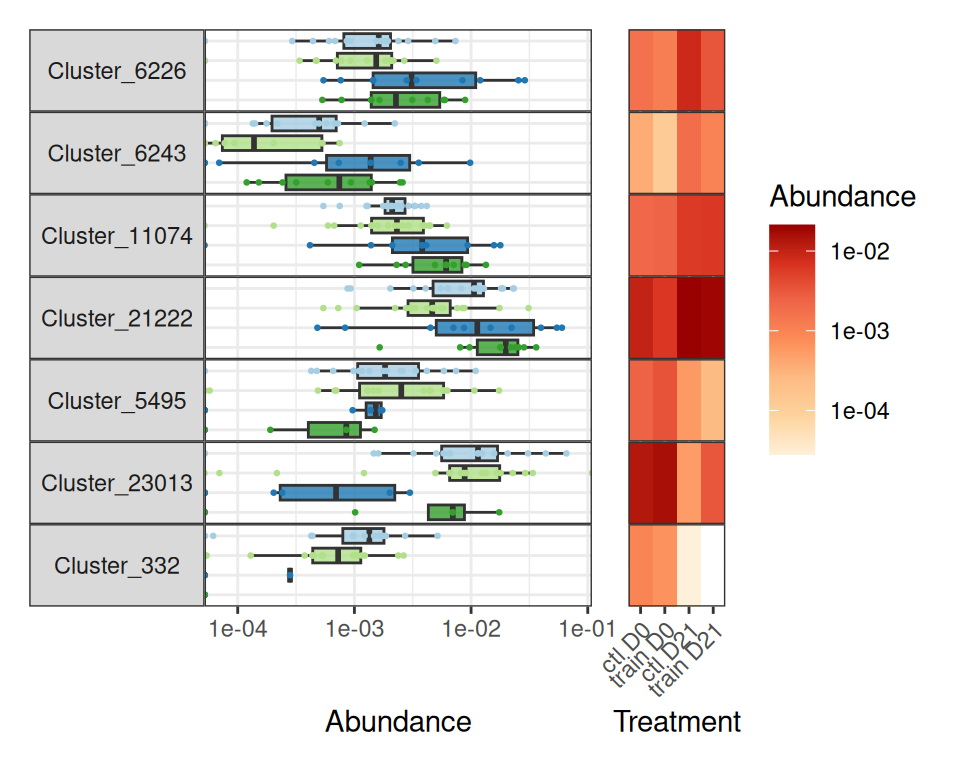
And a closer look at them and their mean abundance (%) in the different treatments show that they are quite minor taxa (at most 2% in a given group).
create_tab_data(physeq = physeq, da_taxa = da_taxa)Association between training performance and microbiota at time D0
We focus here on time point D0 and look at the association between performance increase and microbiota composition. We do so using a PERMANOVA on the Bray-Curtis distance matrix, with MAV, DeltaMAV, Force and DeltaForce as potential structuring factors, without splitting the control and trained groups and without including training as a structuring factor (as it’s already highly correlated with all performance metrics).
performance_ord(physeq, dist_bc, performance = "MAV")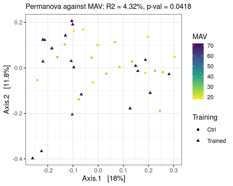
Permutation test for adonis under reduced model
Permutation: free
Number of permutations: 9999

vegan::adonis2(formula = as.formula(glue::glue("subdist ~ {performance}")), data = as_tibble(sample_data(physeq)), permutations = permutations)
         Df SumOfSqs     R2      F Pr(>F)
Model     1   0.2601 0.0432 1.6253 0.0418 *
Residual 36   5.7623 0.9568
Total    37   6.0225 1.0000
---
Signif. codes: 0 '***' 0.001 '**' 0.01 '*' 0.05 '.' 0.1 ' ' 1performance_ord(physeq, dist_bc, performance = "DeltaMAV")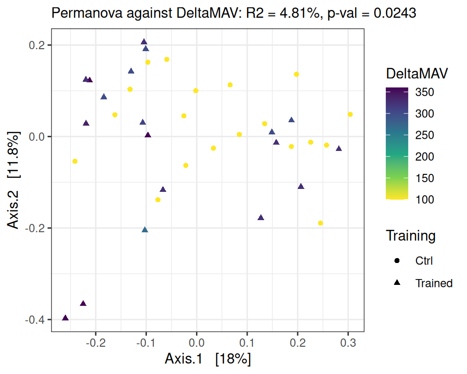
Permutation test for adonis under reduced model
Permutation: free
Number of permutations: 9999

vegan::adonis2(formula = as.formula(glue::glue("subdist ~ {performance}")), data = as_tibble(sample_data(physeq)), permutations = permutations)
         Df SumOfSqs      R2      F Pr(>F)
Model     1   0.2899 0.04813 1.8204 0.0243 *
Residual 36   5.7326 0.95187
Total    37   6.0225 1.00000
---
Signif. codes: 0 '***' 0.001 '**' 0.01 '*' 0.05 '.' 0.1 ' ' 1performance_ord(physeq, dist_bc, performance = "Force")
Permutation test for adonis under reduced model
Permutation: free
Number of permutations: 9999

vegan::adonis2(formula = as.formula(glue::glue("subdist ~ {performance}")), data = as_tibble(sample_data(physeq)), permutations = permutations)
         Df SumOfSqs      R2     F Pr(>F)
Model     1   0.2642 0.04388 1.652 0.0336 *
Residual 36   5.7583 0.95612
Total    37   6.0225 1.00000
---
Signif. codes: 0 '***' 0.001 '**' 0.01 '*' 0.05 '.' 0.1 ' ' 1performance_ord(physeq, dist_bc, performance = "DeltaForce")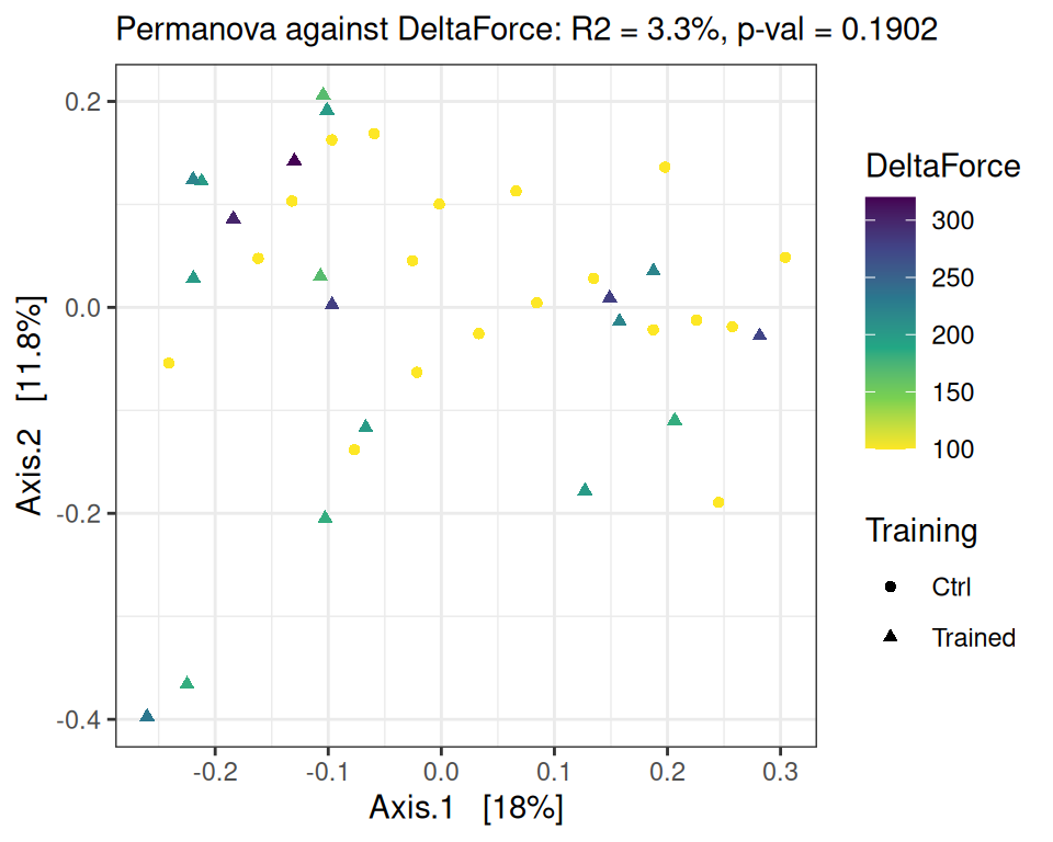
Permutation test for adonis under reduced model
Permutation: free
Number of permutations: 9999

vegan::adonis2(formula = as.formula(glue::glue("subdist ~ {performance}")), data = as_tibble(sample_data(physeq)), permutations = permutations)
         Df SumOfSqs      R2      F Pr(>F)
Model     1   0.1985 0.03296 1.2271 0.1902
Residual 36   5.8240 0.96704
Total    37   6.0225 1.00000
PCA of descriptive data and microbiota changes
We now do a PCA of the descriptive data (understood here as performance metrics) augmented by the following microbiota descriptors:
- scores on the first 3 axis of a PCoA (PCoA1-3) of the microbiota at time D0
- alpha diversity indices (Observed and Shannon) at time D0
Since, we only have performance data at time D0, we focus on those samples only.
desc_data <- div_data |>
  filter(time == "D0") |>
  pivot_wider(names_from = index, values_from = diversity)
pcoa_data <- dist_bc |> as("matrix") %>%
  `[`(desc_data$sample, desc_data$sample) |> as.dist() |>
  cmdscale(k=3) |> `colnames<-`(paste0("PCoA", 1:3)) |>
  as_tibble(rownames = "sample")
pca_data <- inner_join(desc_data, pcoa_data, by = "sample")
pca <- FactoMineR::PCA(pca_data, quali.sup = c(1:8), graph = FALSE)factoextra::fviz_pca_biplot(pca, habillage = "train",
title = "PCA of the performance parameter and microbiota descriptors") +
scale_color_manual(name = "Training", values = train_pal2, labels = c("No Training", "Training")) +
scale_shape_discrete(name = "Training", labels = c("No Training", "Training")) +
theme(legend.position = c(.02, .98), legend.justification = c(0, 1))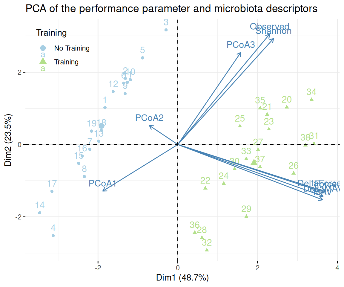
We now do a PCA of the descriptive data (understood here as performance metrics) augmented by the following microbiota descriptors:
- scores on the first 3 axis of a PCoA (PCoA1-3) of the microbiota at times D0 and D21
- alpha diversity indices (Observed and Shannon) at times D0 and D21
Since we only have performance data at time D0, we only use performance metrics at time D0 and we limit the PCA to mice for which we have microbial data at both times D0 and D21.
create_pcoa_data <- function(desc_data, suffix = "_D0") {
  inner_join(
    desc_data,
    dist_bc |> as("matrix") %>%
      `[`(desc_data$sample, desc_data$sample) |> as.dist() |>
      cmdscale(k=3) |> `colnames<-`(paste0("PCoA", 1:3, suffix)) |>
      as_tibble(rownames = "sample"),
    by = "sample"
  )
}
create_desc_data <- function(...) {
  div_data |>
  filter(...) |>
  pivot_wider(names_from = index, values_from = diversity)
}
pca_data <- inner_join(
  create_desc_data(time == "D0") |> create_pcoa_data(),
  create_desc_data(time == "D21") |> create_pcoa_data(suffix = "_D21") |> select(animalID, Observed, Shannon, ends_with("_D21")),
  by = join_by(animalID), suffix = c("_D0", "_D21")
)
pca <- FactoMineR::PCA(pca_data, quali.sup = c(1:8), graph = FALSE)factoextra::fviz_pca_biplot(pca, habillage = "train",
title = "PCA of the performance parameter and microbiota descriptors") +
scale_color_manual(name = "Training", values = train_pal2, labels = c("No Training", "Training")) +
scale_shape_discrete(name = "Training", labels = c("No Training", "Training")) +
theme(legend.position = "inside", legend.position.inside = c(1, 0),
legend.justification = c(1, 0))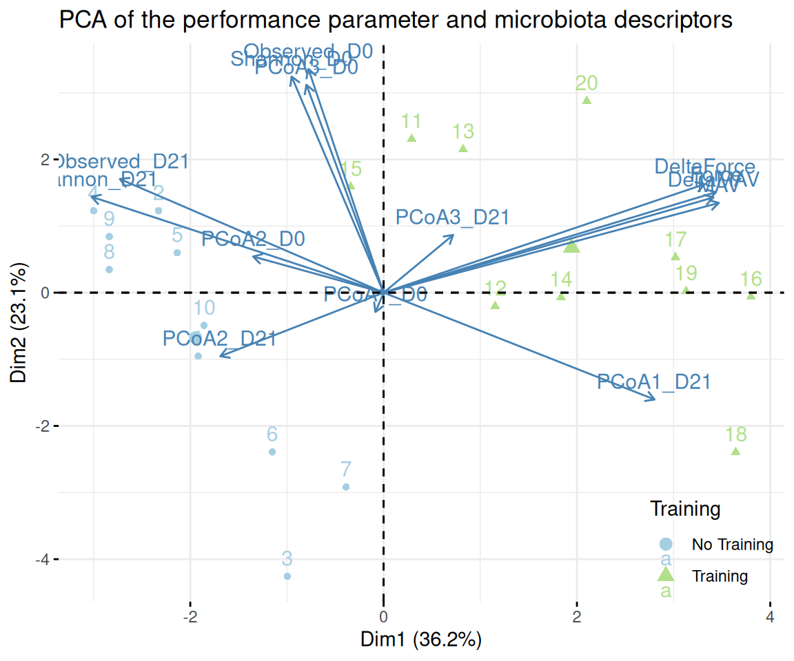
We can repeat the PCA analyses on the trained mice only and highlight the responder versus the resistant to suspension.
We see that the separation between responder and resistant is highly associated to the first PCA, which is itself highly associated to microbial descriptor, chief among which are the alpha diversity (higher in resistant mice) and the first PCoA at times D0 and D21 (this is not surprising as responders and resistants were defined that way).
The only performance indicator associated to axis 1 is the MAV.
pca <- FactoMineR::PCA(pca_data |> filter(training) |>
                         mutate(responder = if_else(animalID %in% paste0("T", c(14, 16:19)), "responder", "resistant"),
                                .after = treatment),
quali.sup = c(1:9), graph = FALSE)factoextra::fviz_pca_biplot(pca, habillage = "responder",
title = "PCA of the performance parameter and microbiota descriptors") +
theme(legend.position = "inside", legend.position.inside = c(1, 0),
legend.justification = c(1, 0))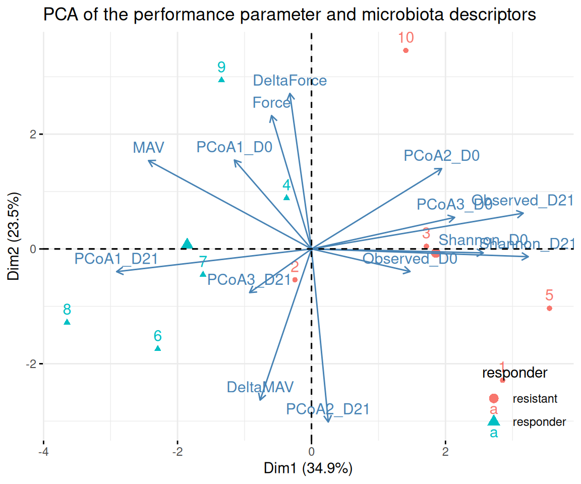
Responders versus resistant to suspension.
We now compare responder to resistant mice. We define responder mice as trained mice for which the change in the PCoA1 coordinate after suspension is greater than 0.1. There are 5 such mice: T14, T16, T17, T18 and T19.
We first add this status to the dataset
physeq_train <- subset_samples(physeq, animalID %in% paste0("T", 11:20)) %>%
  prune_taxa(taxa_sums(.) > 0, .)
sample_data(physeq_train)$responder <- if_else(
  get_variable(physeq_train, "animalID") %in% paste0("T", c(14, 16:19)),
  "Responder", "Resistant"
)
p + facet_nested(~ responder + time, scales="free_x", space = "free_x") +
theme(legend.position = "bottom")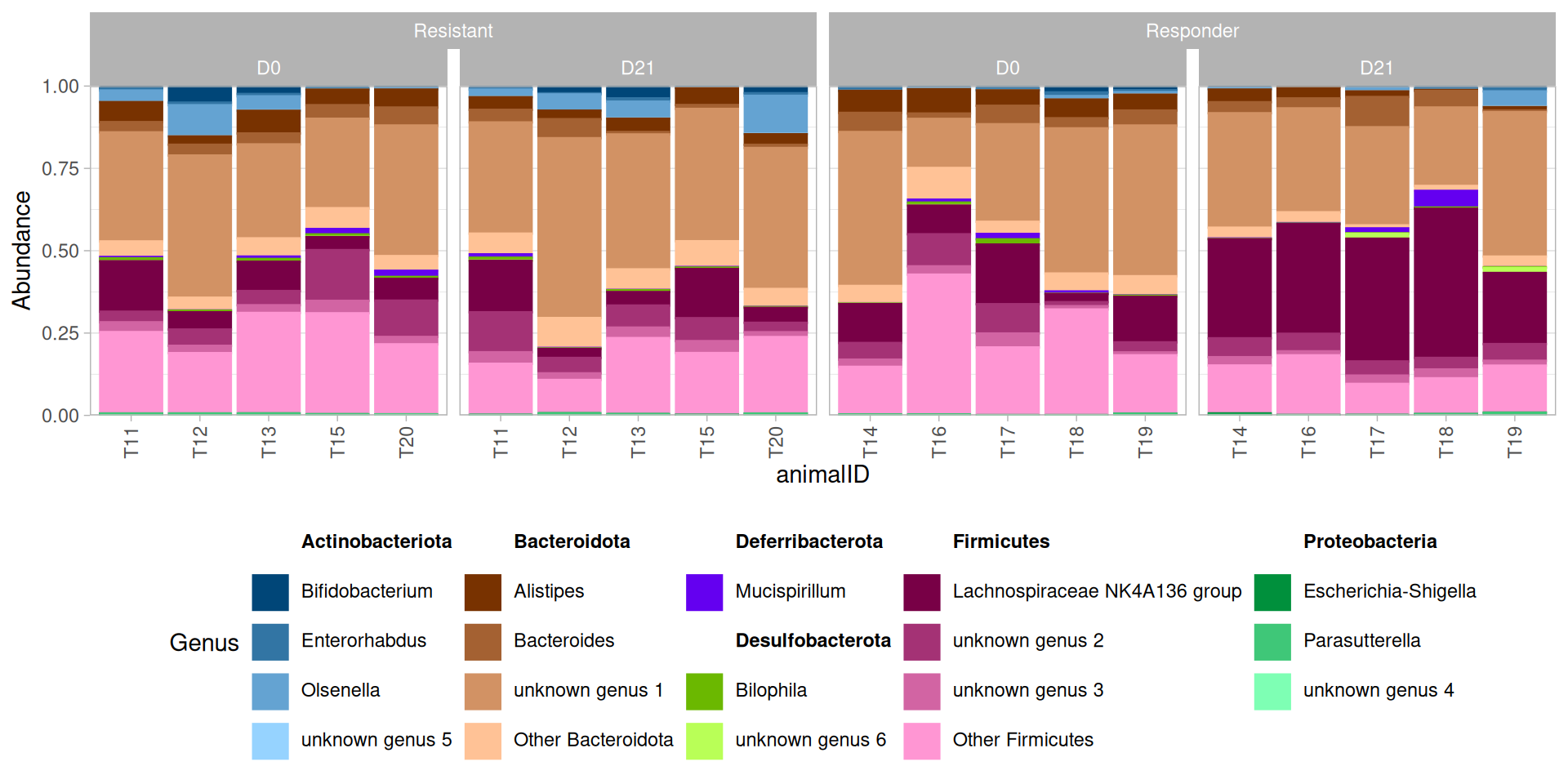
There seems to be a huge increase after suspension in the Lachnospiraceae NK4A136 group in the responders. Zooming in on this genus, we find that both the abundance of and the composition within this genus differs between the two responders and non-responders.
plot_composition(physeq_train, taxaRank1 = "Genus", x = "animalID",
                 taxaSet1 = "Lachnospiraceae NK4A136 group", taxaRank2 = "ASV") +
  facet_nested(~ responder + time, scales="free_x", space = "free_x") +
  theme(legend.position = "bottom")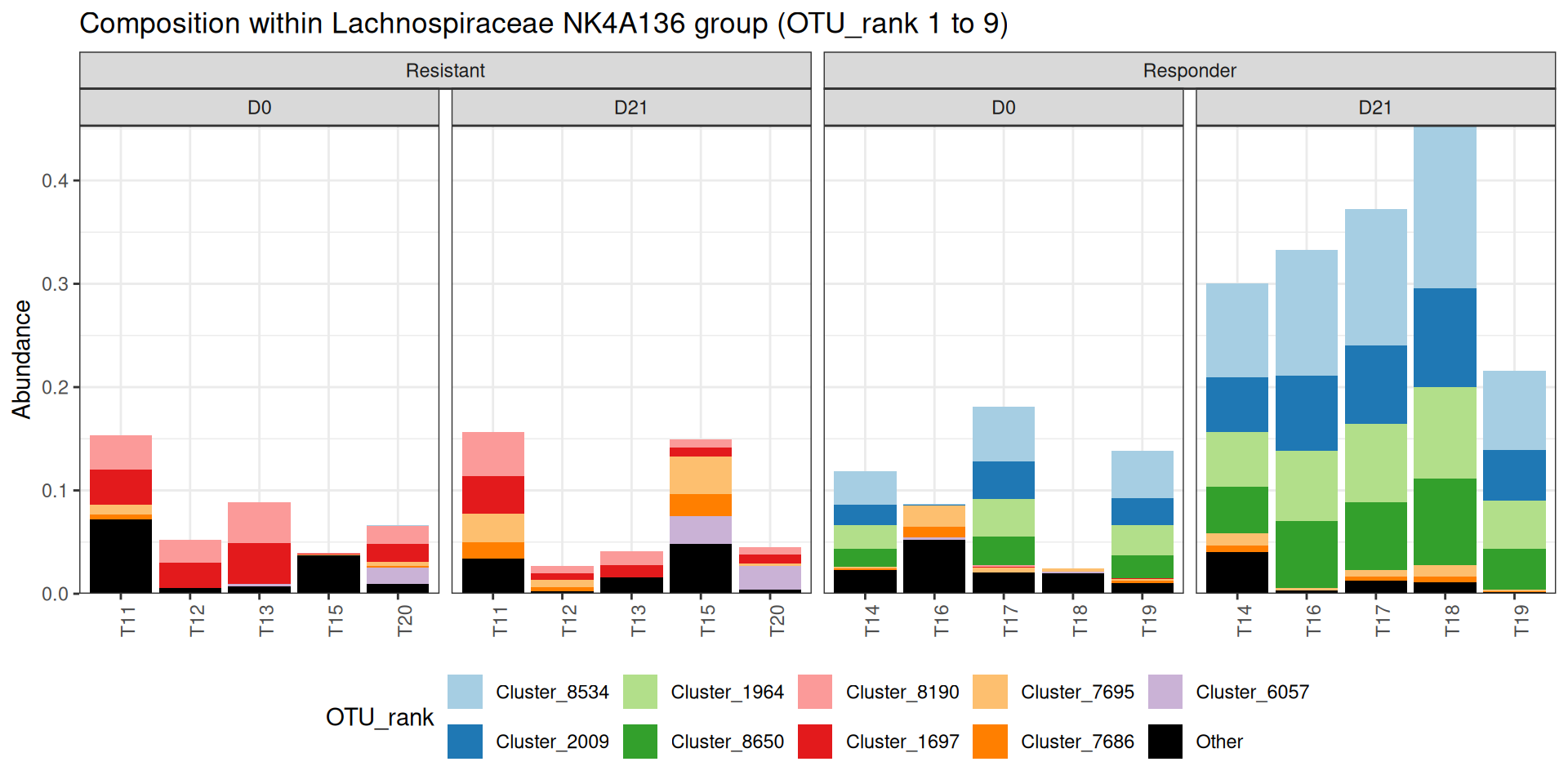
To explore this further, we do a differential analysis on time, responder status and their interaction. We look specifically at two sets of taxa:
- those who have a significant time:status interaction.
- those who change between D0 and D21 in the responder group
- those who change between D0 and D21 in the resistant group
da_taxa_responder <- create_da_taxa_responder(physeq_train)create_da_plot(physeq_train, da_taxa_responder)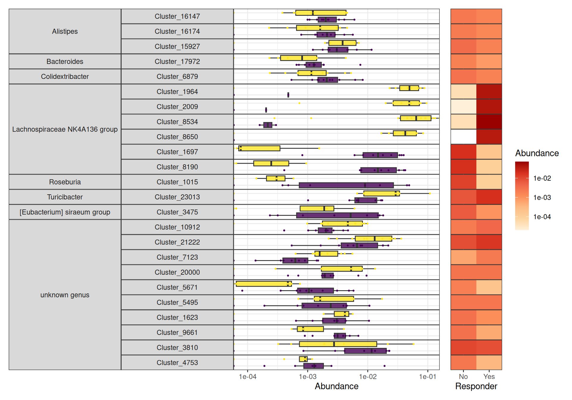
create_tab_data(physeq_train, da_taxa_responder)For the differential analysis in the responder mice group, because of the limited sample size (5 mice only), the set of differential taxa consists almost only of ASV that are always present at time D0 and absent at time D21 or vice versa.
da_taxa_responder_time <- create_da_taxa_time(physeq_train, responder = "Responder")  |>
  filter(padj <= 0.07) |>
mutate(OTU = fct_drop(OTU))create_da_plot_time(physeq_train, da_taxa_responder_time, responder = "Responder")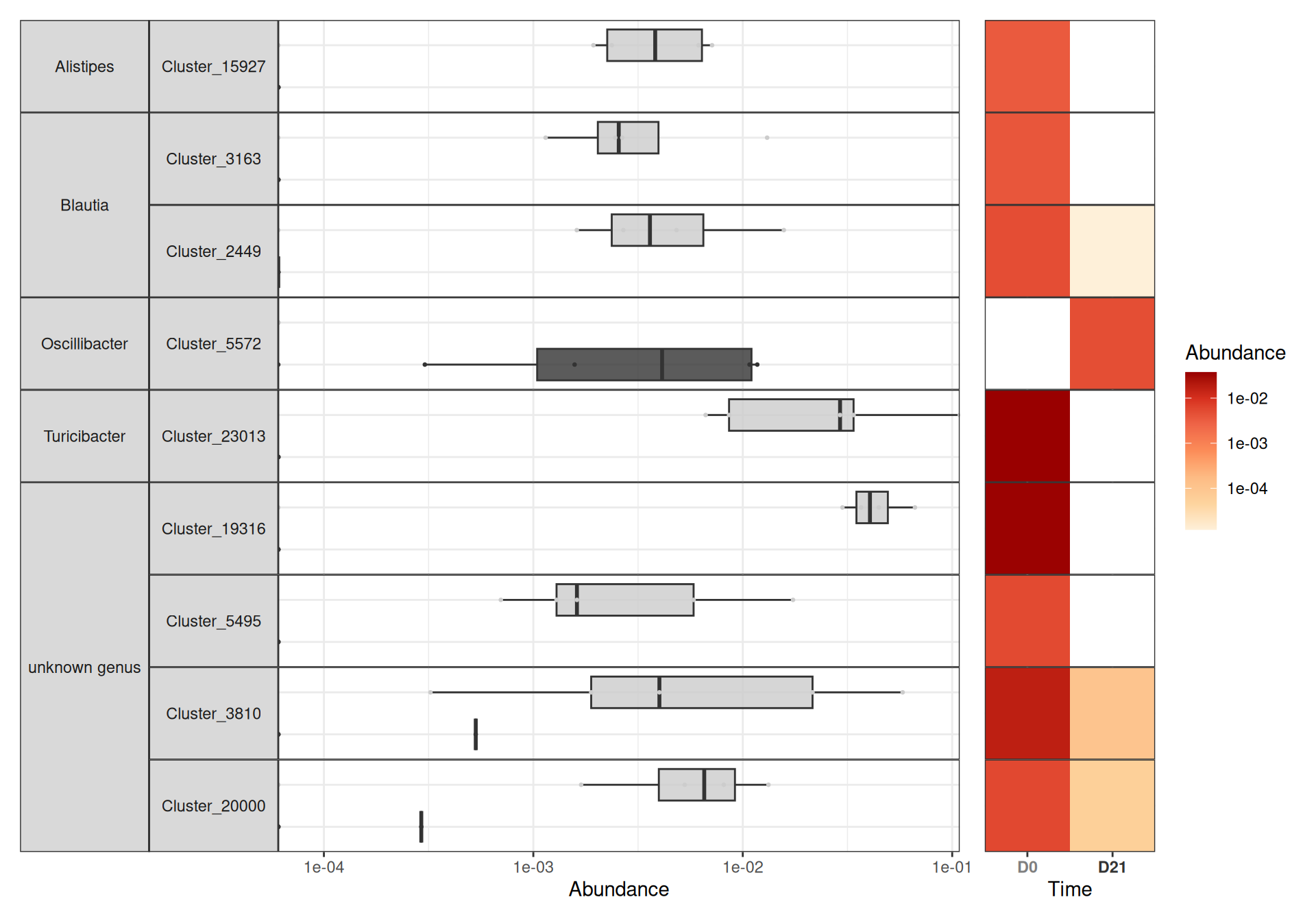
create_tab_data_time(physeq_train, da_taxa_responder_time, responder = "Responder")For the differential analysis in the resistant mice group, because of the limited sample size (5 mice only), the set of differential taxa consists almost only of ASV that are always present at time D0 and absent at time D21 or vice versa.
da_taxa_resistant_time <- create_da_taxa_time(physeq_train, responder = "Resistant") |>
  filter(padj <= 0.07) |>
mutate(OTU = fct_drop(OTU))create_da_plot_time(physeq_train, da_taxa_resistant_time, responder = "Resistant")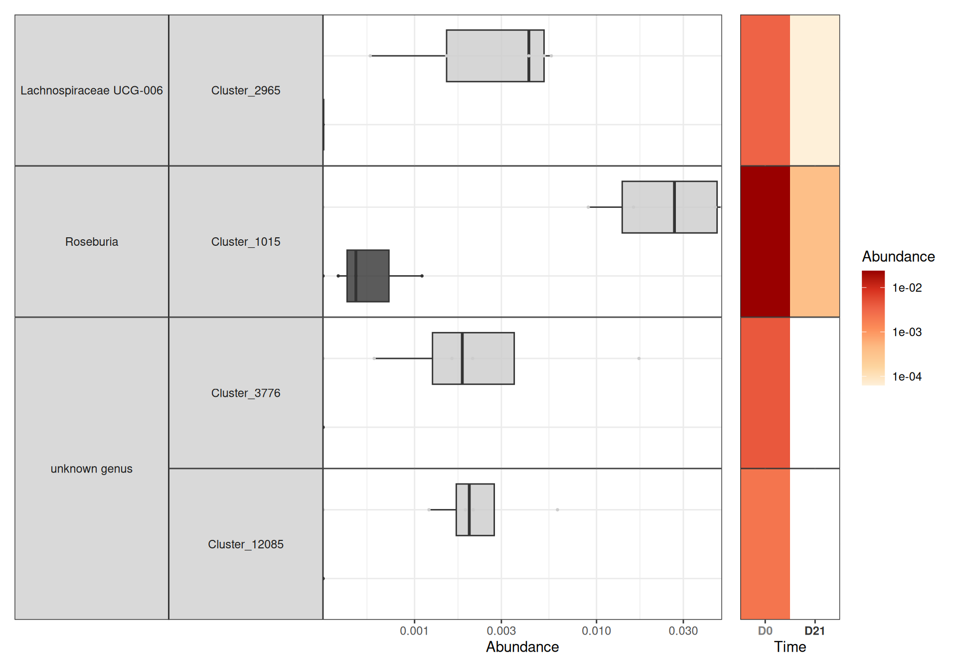
create_tab_data_time(physeq_train, da_taxa_resistant_time, responder = "Resistant")Focus on specific bacteria
The bacteria Parabacteroides distasonis and Barnesiella sp. could not be found in the dataset (although they are present in the Silva database).
References
1. Shen W, Le S, Li Y, Hu F. SeqKit: A cross-platform and ultrafast toolkit for FASTA/q file manipulation. PloS one. 2016;11:e0163962.
2. Andrews S. FastQC a quality control tool for high throughput sequence data. http://www.bioinformatics.babraham.ac.uk/projects/fastqc/. 2010. http://www.bioinformatics.babraham.ac.uk/projects/fastqc/.
3. Ewels P, Magnusson M, Lundin S, Käller M. MultiQC: Summarize analysis results for multiple tools and samples in a single report. Bioinformatics. 2016;32:3047–8.
4. Escudié F, Auer L, Bernard M, Mariadassou M, Cauquil L, Vidal K, et al. FROGS: Find, Rapidly, OTUs with Galaxy Solution. Bioinformatics. 2018;34:1287–94. doi:10.1093/bioinformatics/btx791.
5. Bernard M, Rué O, Mariadassou M, Pascal G. FROGS: a powerful tool to analyse the diversity of fungi with special management of internal transcribed spacers. Briefings in Bioinformatics. 2021;22. doi:10.1093/bib/bbab318.
6. Callahan BJ, McMurdie PJ, Rosen MJ, Han AW, Johnson AJA, Holmes SP. DADA2: High-resolution sample inference from illumina amplicon data. Nature methods. 2016;13:581.
7. Altschul SF, Gish W, Miller W, Myers EW, Lipman DJ. Basic local alignment search tool. Journal of molecular biology. 1990;215:403–10.
8. Quast C, Pruesse E, Yilmaz P, Gerken J, Schweer T, Yarza P, et al. The SILVA ribosomal RNA gene database project: Improved data processing and web-based tools. Nucleic acids research. 2012;41:D590–6.
Reuse
This document will not be accessible without prior agreement of the partners