#library(DT)library(tidyverse)library(kableExtra)library(phyloseq)library(phyloseq.extended)library(data.table)library(InraeThemes)library(readr) #read_delimlibrary(ggplot2) # graphicslibrary(microbiome) # for boxplot_alpha functionlibrary(mia) # microbiome analysis with SummarizedExperiment and TreeSummarizedExperimentlibrary(emmeans) #post hoc testslibrary(reactable) #table formatting and stylinglibrary(reactablefmtr) #table formatting and stylinglibrary(openxlsx) #save results to excel sheetslibrary(metacoder) # differential abundancelibrary(ggtree) # visualizationlibrary(ggtreeExtra) # visualizationlibrary(ComplexHeatmap) # produce heatmaplibrary(microViz) # analysis and visualization of microbiome sequencing data
Note
This document is a report of the analyses performed. You will find all the code used to analyze these data. The version of the tools (maybe in code chunks) and their references are indicated, for questions of reproducibility.
Aim of the project
Influence of treatment antibiotics in a murine model of infection with Clostridium difficile (ICD). Injection of C. difficile were performed at J00 and J37.
Différencier les groupes ctrl et traités aux antibiotiques (VAN, MTZ, FDX, R = réinfections multiples), et comparer les cinétiques entre les groupes. Les échantillons contrôle sont infectés mais pas traités aux antibiotiques.
Etudier les cinétiques au sein des traitements (CTRL, VAN, MTZ, FDX, R). Est-ce qu’il y a un retour à J-6 ? Clairance de la bactérie (zéro dans les fécès, attention biofilm et sporulation peuvent encore existés)
All data is managed by the migale facility for the duration of the project. Once the project is over, the Migale facility does not keep your data. We will provide you with the raw data and associated metadata that will be deposited on public repositories before the results are used. We can guide you in the submission process. We will then decide which files to keep, knowing that this report will also be provided to you and that the analyses can be replayed if needed.
Analyses
Experiment
Fig1: Experimental protocol
Phyloseq rarefied data with all samples
Show the code
frogs <-readRDS(file ="../html/frogs.rds")
For having the same sampling depth for all samples, we rarefy them before exploring the diversity.
Note that the rarefaction was performed on all samples from the complete study. We extracted samples of interest from the frogs_rare phyloseq object to calculate alpha diversity. Alpha diversity is calculated within sample and do not change with the previous analyses on the complete study.
Show the code
frogs_rare_withoutR <-subset_samples(frogs_rare, GROUP !="R")
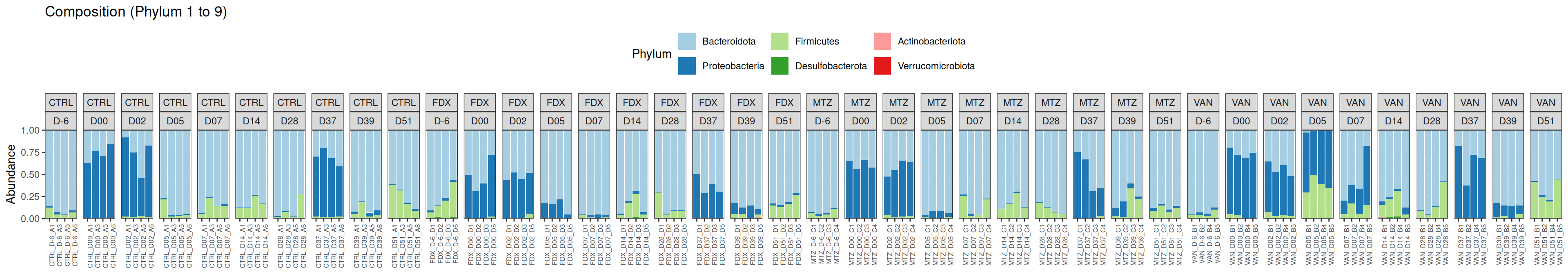
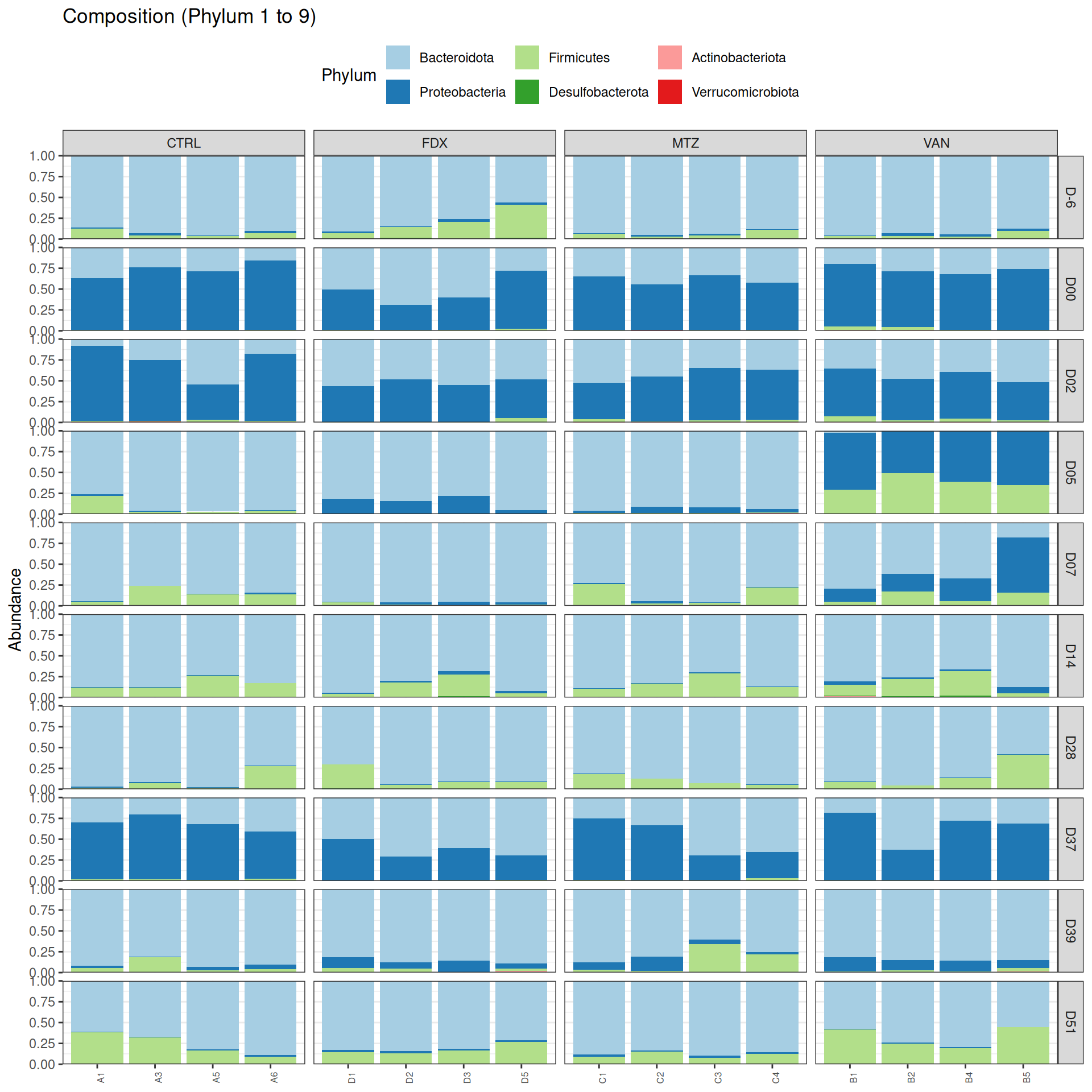
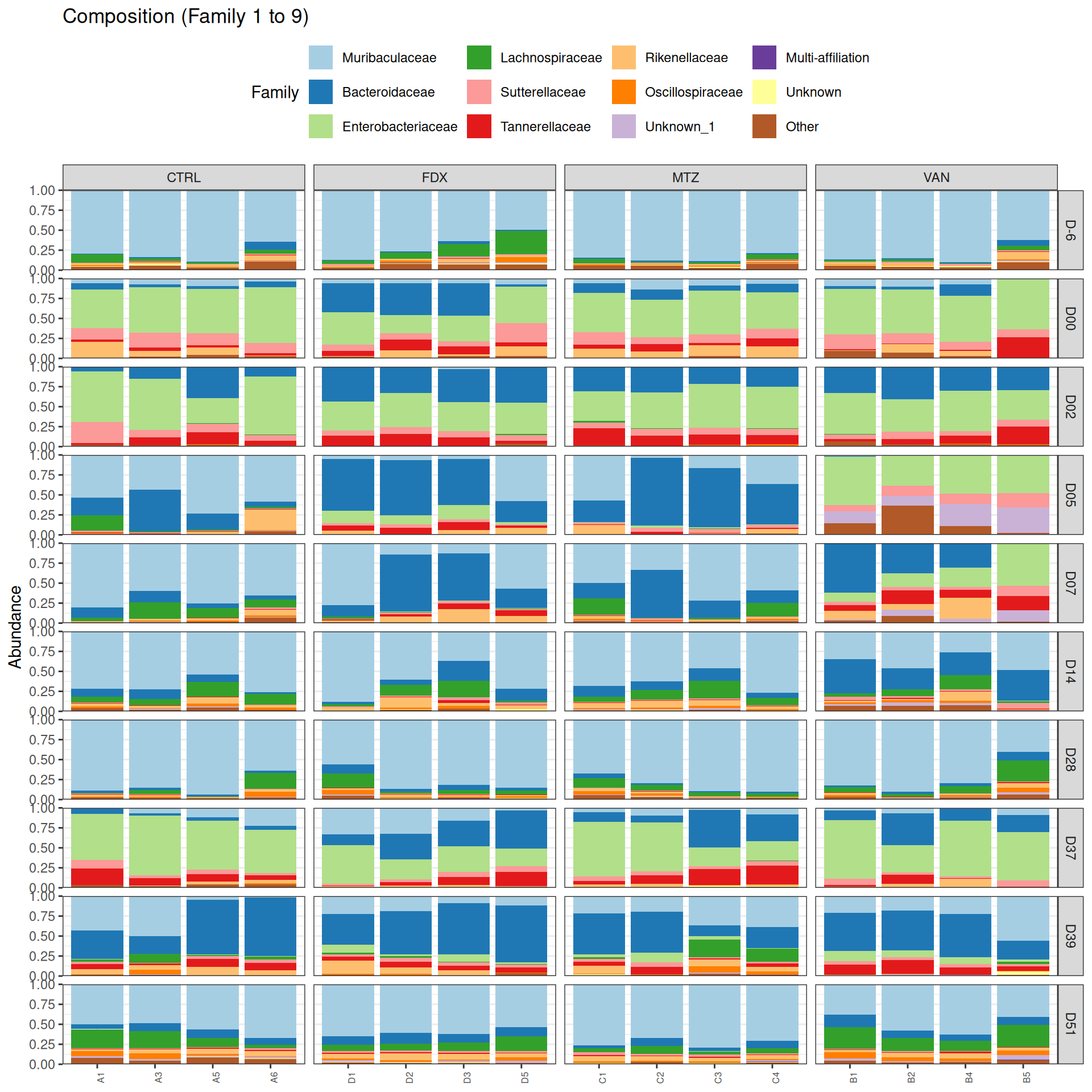
Taxonomic composition
After rarefaction, let’s have a look at the Phylum and genus levels composition with two types of plot.
Problematic taxa
                 taxa  Kingdom     Phylum      Class                      Order
Cluster_27 Cluster_27 Bacteria Firmicutes Clostridia Clostridia vadinBB60 group
            Family rank
Cluster_27 Unknown    9
#model <- aov(Observed ~ DAY*GROUP, data = div_data)#anova(model)#coef(model)# produce parwise comparison test with Tukey's post-hoc correction #TukeyHSD(model, which ="DAY:GROUP")alphadiv.lm <-lm(Observed ~ DAY*GROUP, data = div_data)anova(alphadiv.lm)
Analysis of Variance Table

Response: Observed
           Df Sum Sq Mean Sq F value    Pr(>F)
DAY         9 469628   52181 218.935 < 2.2e-16 ***
GROUP       3  13905    4635  19.447 2.423e-10 ***
DAY:GROUP  27  33932    1257   5.273 8.762e-11 ***
Residuals 120  28601     238
---
Signif. codes:  0 '***' 0.001 '**' 0.01 '*' 0.05 '.' 0.1 ' ' 1
Show the code
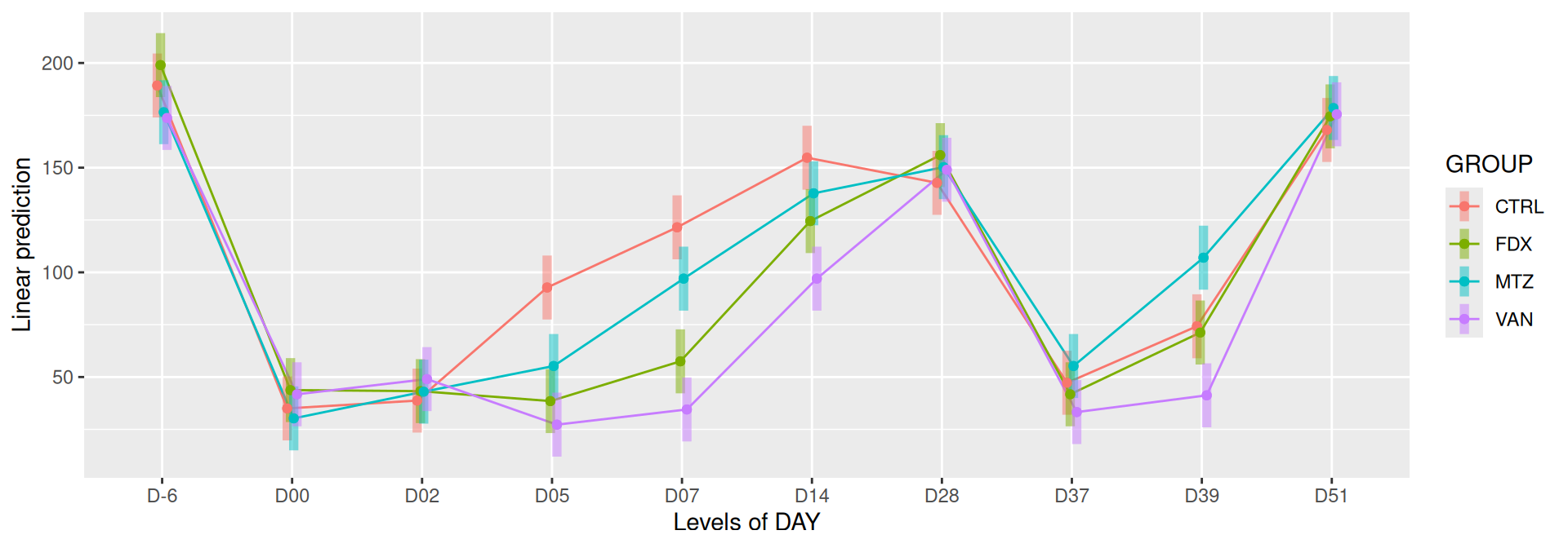
# interaction visualisationpar(mfrow =c(1,2))emmip(alphadiv.lm, GROUP ~ DAY, CIs =TRUE)
Show the code
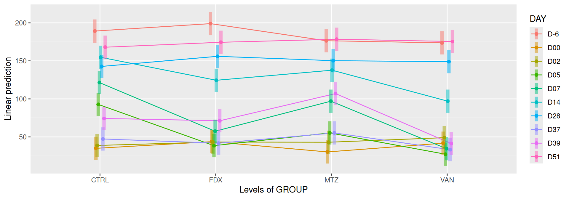
emmip(alphadiv.lm, DAY ~ GROUP, CIs =TRUE)
Show the code
par(mfrow =c(1,1))#tests EMM <-emmeans(alphadiv.lm, ~ DAY*GROUP)# tests correction are performed within the variable# P value adjustment: tukey method for comparing a family of 12 estimatescomp1 <-pairs(EMM, simple ="DAY")# P value adjustment: tukey method for comparing a family of 5 estimates comp2 <-pairs(EMM, simple ="GROUP")
Show the code
# P value adjustment: tukey method for comparing a family of 60 estimatesres_emm <-contrast(EMM, method ="revpairwise", by =NULL,enhance.levels =c("DAY", "GROUP"), adjust ="tukey")
Important
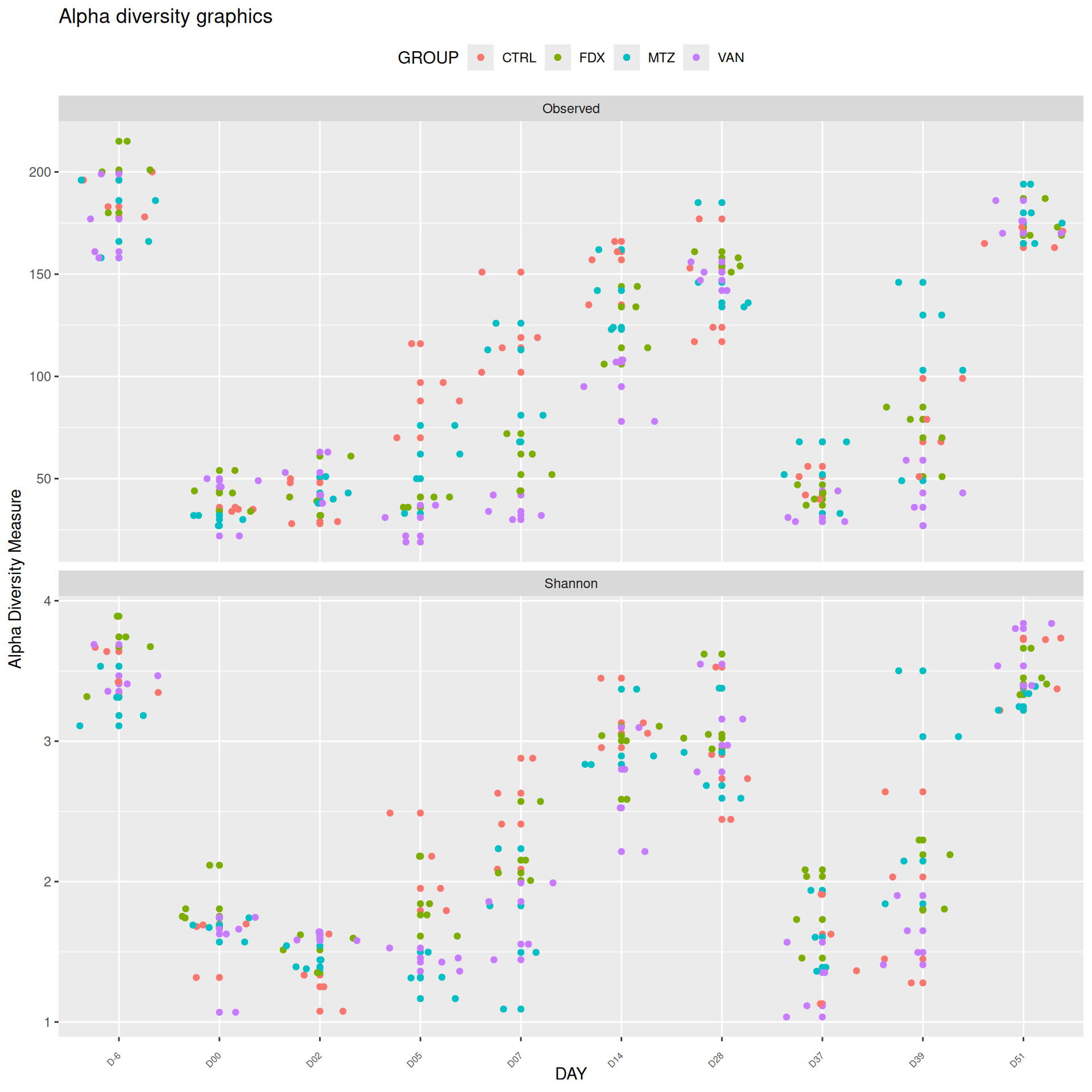
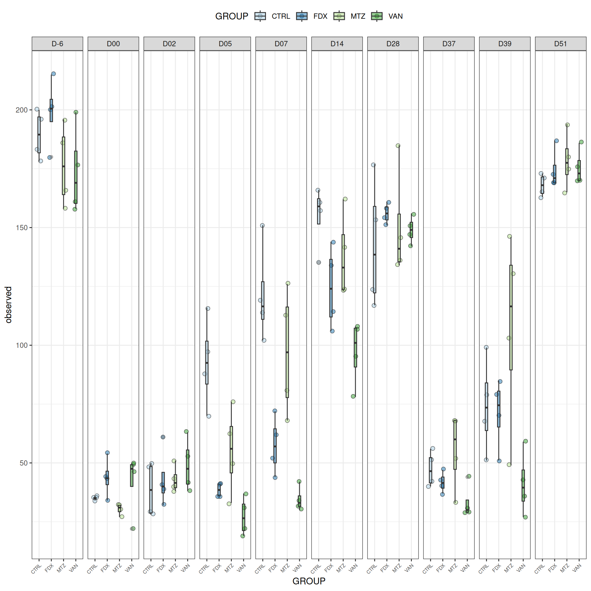
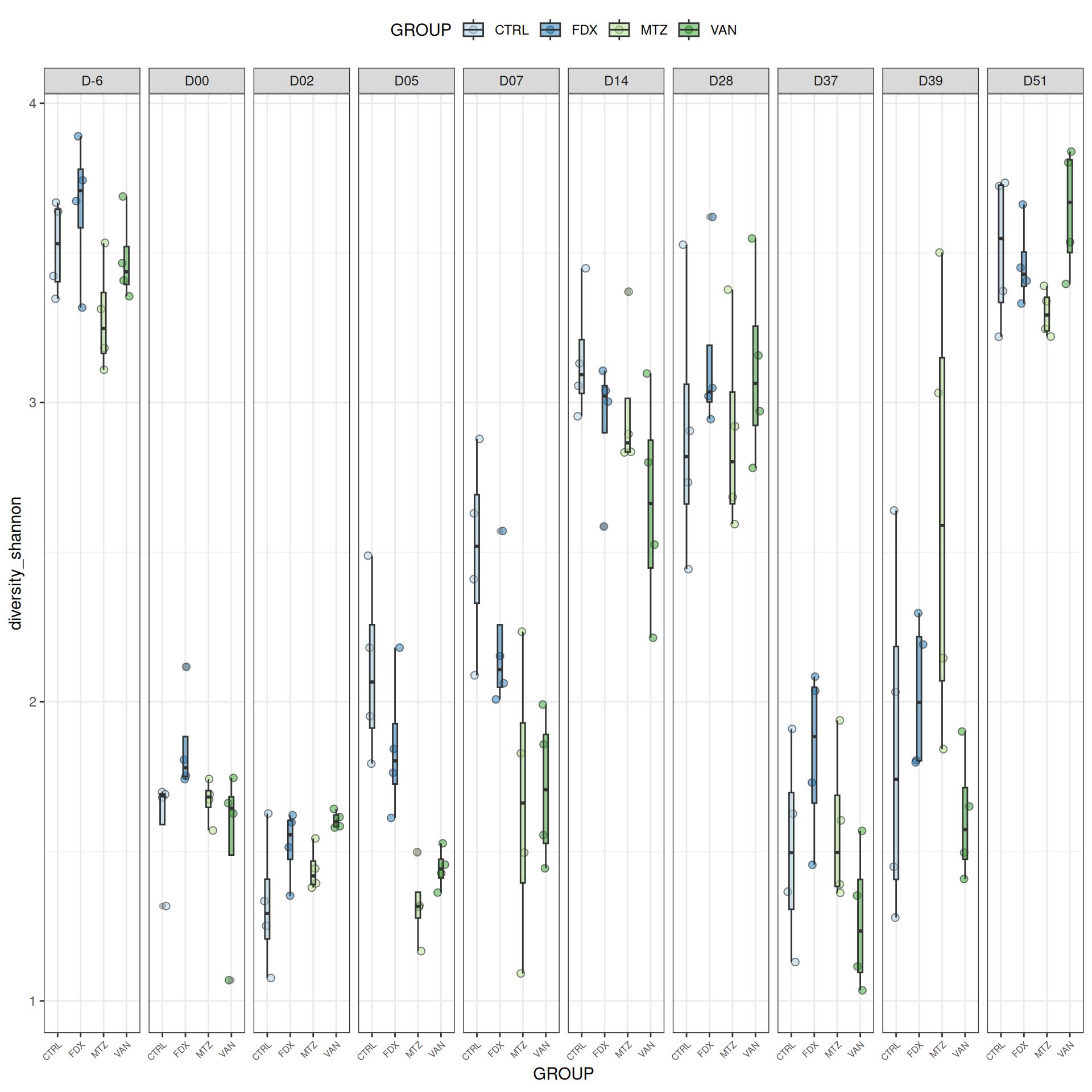
Richness is significantly different by DAY, GROUP and the interaction DAY:GROUP. Pairwise tests between DAY and GROUP were performed with post hoc Tukey’s test to determine which were significant. We observed differences between the GROUP treatments at D05, D07, D14 and also at D39 in other way.
Beta-diversity on subset excluding R treatment
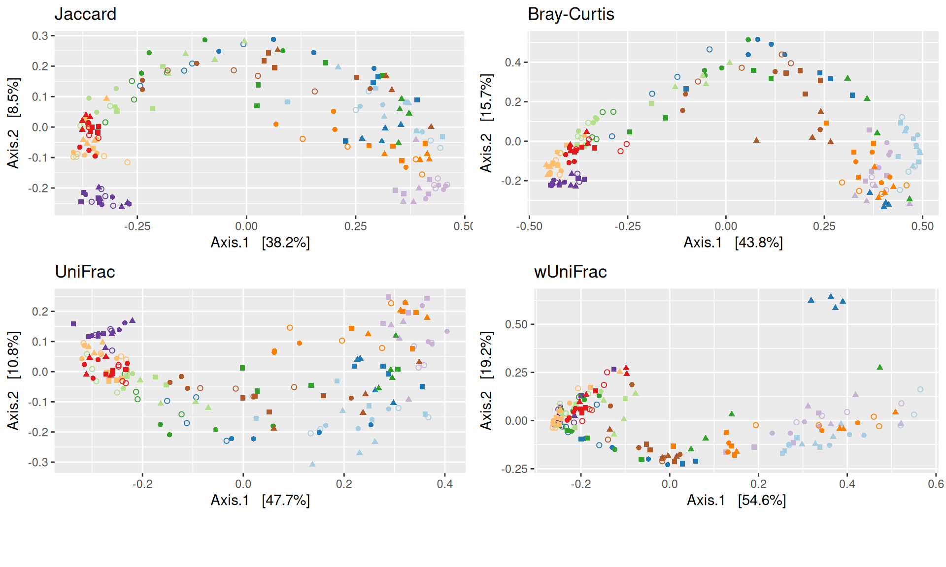
The dissimilarity between samples based on taxonomic composition is calculated with one of these Beta diversities: Bray-Curtis, Unweighted and weighted Unifrac, Jaccard index. The Jaccard index uses presence/absence information only whereas UniFrac integrates information from the phylogenetic tree.
Show the code
# use all samples from the complete study frogs_raredist.jac <- phyloseq::distance(frogs_rare, method ="cc")dist.bc <- phyloseq::distance(frogs_rare, method ="bray")dist.uf <- phyloseq::distance(frogs_rare, method ="unifrac")dist.wuf <- phyloseq::distance(frogs_rare, method ="wunifrac")distance_list <-list("Jaccard"= dist.jac,"Bray-Curtis"= dist.bc,"UniFrac"= dist.uf,"wUniFrac"= dist.wuf)
# Mahendra's function# used own color's palette and shapemy_pcoa_with_arrows2 <-function(physeq = mydata_rare, variable1, variable2, shapeval, colorpal) {# select samples of interest where all samples were used to calculate the distances between samples # dist.jac is previously calculated with all samples of the study#dist.c <- phyloseq::distance(physeq, "jaccard")#dist.c <- dist.jac %>% as.matrix() %>% `[`(sample_names(physeq), sample_names(physeq)) %>% as.dist() dist.c <- dist.bc %>%as.matrix() %>%`[`(sample_names(physeq), sample_names(physeq)) %>%as.dist() ord.c <-ordinate(physeq, "MDS", dist.c) p <-plot_ordination(physeq, ord.c)# ## Build arrow data plot_data <- p$data arrow_data <- plot_data %>%group_by(pick({{variable2}}, {{variable1}})) %>%arrange({{variable1}}) %>%mutate(xend = Axis.1, xstart =lag(xend),yend = Axis.2, ystart =lag(yend) )## Plot with arrows p +aes(shape = .data[[ variable2 ]], color = .data[[ variable1 ]]) +scale_shape_manual(values = shapeval) +scale_color_manual(name = colorpal$name,labels = colorpal$labels,values = colorpal$values) +theme_bw() +geom_segment(data = arrow_data,aes(x = xstart, y = ystart, xend = xend, yend = yend),size =0.8, linetype ="3131",arrow =arrow(length=unit(0.1,"inches")),show.legend =FALSE) +geom_point(size =3) +theme(legend.position ="bottom")}
Show the code
# MDS plot for samples of interests # from distance calculated with all samples of the complete study# used https://colorbrewer2.org/#type=qualitative&scheme=Paired&n=12Jour_pal <-list(name ="DAY",labels =c("D-6", "D00", "D02", "D05", "D07", "D14", "D28", "D37", "D39", "D51"),values =c("#6a3d9a", "#cab2d6", "#a6cee3", "#1f78b4", "#33a02c", "#b2df8a", "#fdbf6f", "#ff7f00", "#b15928", "#e31a1c"))GROUP_shape <-list(values =c(1, 15, 16, 17))my_plot2(variable1 ="DAY",variable2 ="GROUP",physeq = frogs_rare_withoutR,shapeval = GROUP_shape$values,colorpal = Jour_pal )
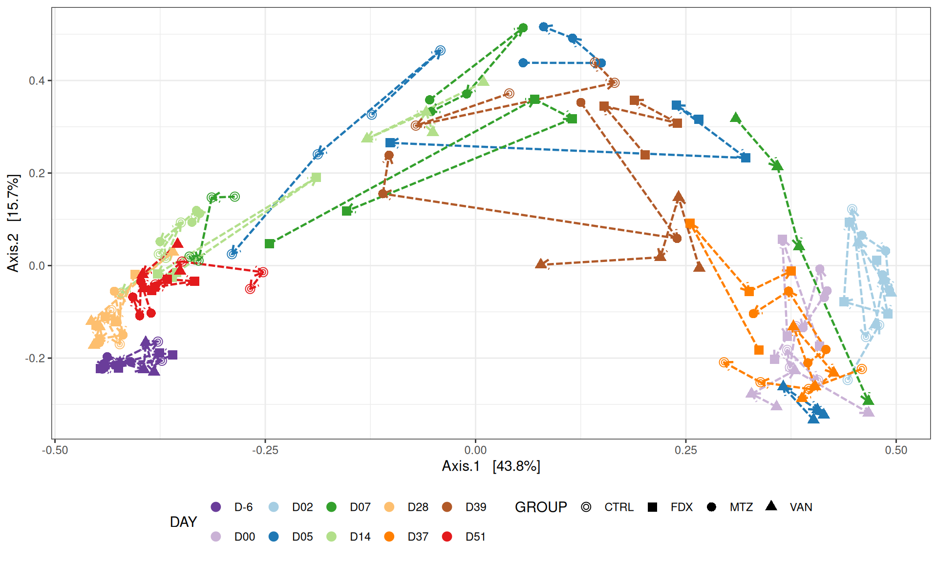
The percentage of variance explained on the first two axes of the MDS plot is 59.5% (=43.8 + 15.7) and 46.5% (=38 +8.5) for the Bray-Curtis and Jaccard distances, respectively. We use the Bray-Curtis’s distance and show MDS trajectories of the communities intra conditions.
Show the code
# MDS plot for samples of interests # from distance calculated with all samples of the complete study# used https://colorbrewer2.org/#type=qualitative&scheme=Paired&n=12Jour_pal <-list(name ="DAY",labels =c("D-6", "D00", "D02", "D05", "D07", "D14", "D28", "D37", "D39", "D51"),values =c("#6a3d9a", "#cab2d6", "#a6cee3", "#1f78b4", "#33a02c", "#b2df8a", "#fdbf6f", "#ff7f00", "#b15928", "#e31a1c"))GROUP_shape <-list(values =c(1, 15, 16, 17))p <-my_pcoa_with_arrows2(variable1 ="DAY",variable2 ="GROUP",physeq = frogs_rare_withoutR,shapeval = GROUP_shape$values,colorpal = Jour_pal)p
Important
The multidimensional scaling (MDS / PCoA) showed that the samples were distributed according to the variable DAY and the evolution of the infection on the two first axes. The samples from D-6, D28 and D51 are close to each other, and opposite to those from D00, D02 and D37 on the first axis. The microbiota composition depends on the DAY and GROUP treatment which is reflected by the variability on the two axes. The differences between the GROUP treatments are more visible at D05, D07, D14 and also at D39.
Permutation test for adonis under reduced model
Permutation: free
Number of permutations: 9999

vegan::adonis2(formula = dist.c ~ DAY * GROUP, data = metadata, permutations = 9999)
          Df SumOfSqs      R2      F Pr(>F)
Model     39   37.281 0.81061 13.169  1e-04 ***
Residual 120    8.710 0.18939
Total    159   45.991 1.00000
---
Signif. codes:  0 '***' 0.001 '**' 0.01 '*' 0.05 '.' 0.1 ' ' 1
Important
The change in microbiota composition measured by the Bray-Curtis Beta diversity is significantly different between DAY, GROUP and also between the levels of the interaction factor DAY:GROUP at 0.05 significance level. The influence of the factors differs between ecosystems.
Show the code
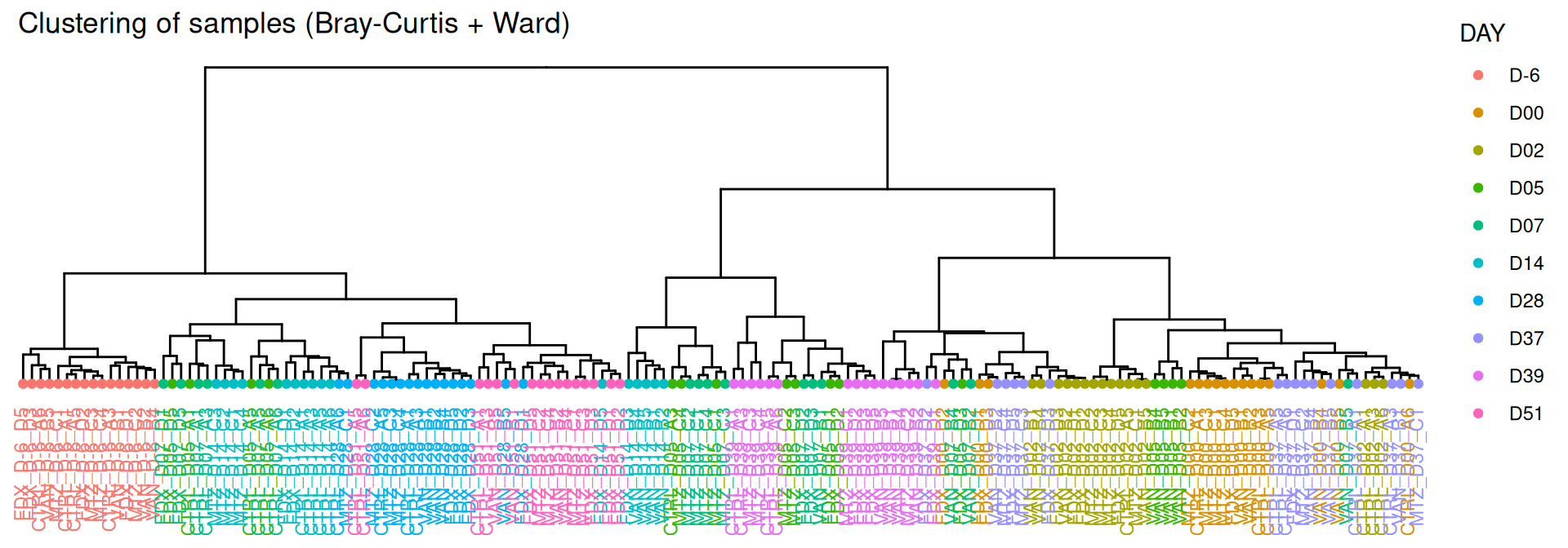
par(mfrow=c(1,1))par(mar =c(3, 0, 2, 0), cex =0.7)phyloseq.extended::plot_clust(frogs_rare_withoutR, dist ="bray", method ="ward.D2", color ="DAY",title ="Clustering of samples (Bray-Curtis + Ward)")
Show the code
# phyloseq.extended::plot_clust(frogs_rare_withoutR, dist = "jaccard", method = "ward.D2", color = "DAY",# title = "Clustering of samples (Jaccard + Ward)")
Important
Hierarchical clustering based on the Bray-Curtis dissimilarity and the Ward aggregation criterion shows that sample composition is not entirely structured by DAY. Groups were formed according to the date of infection and the existing DAY:GROUP interaction.
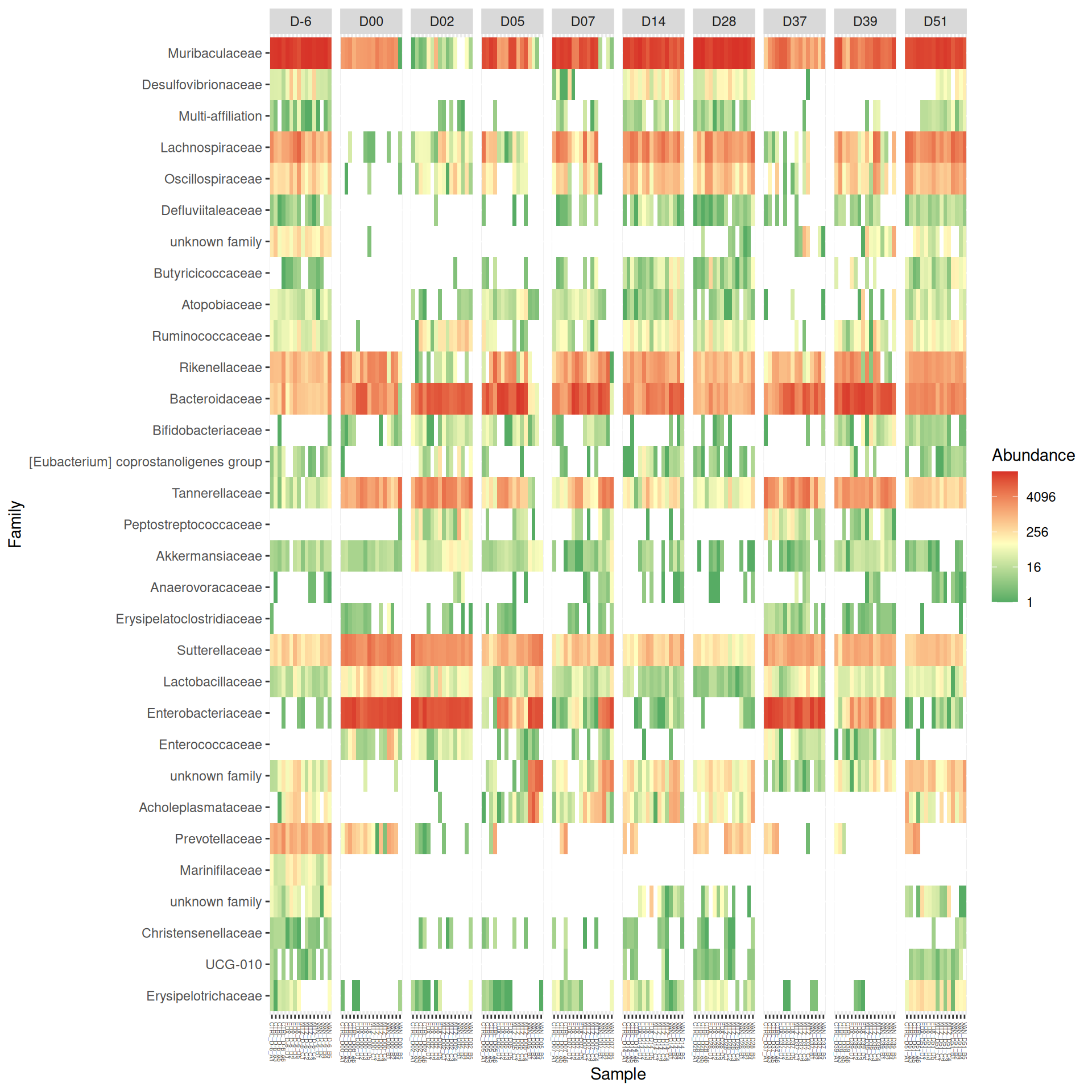
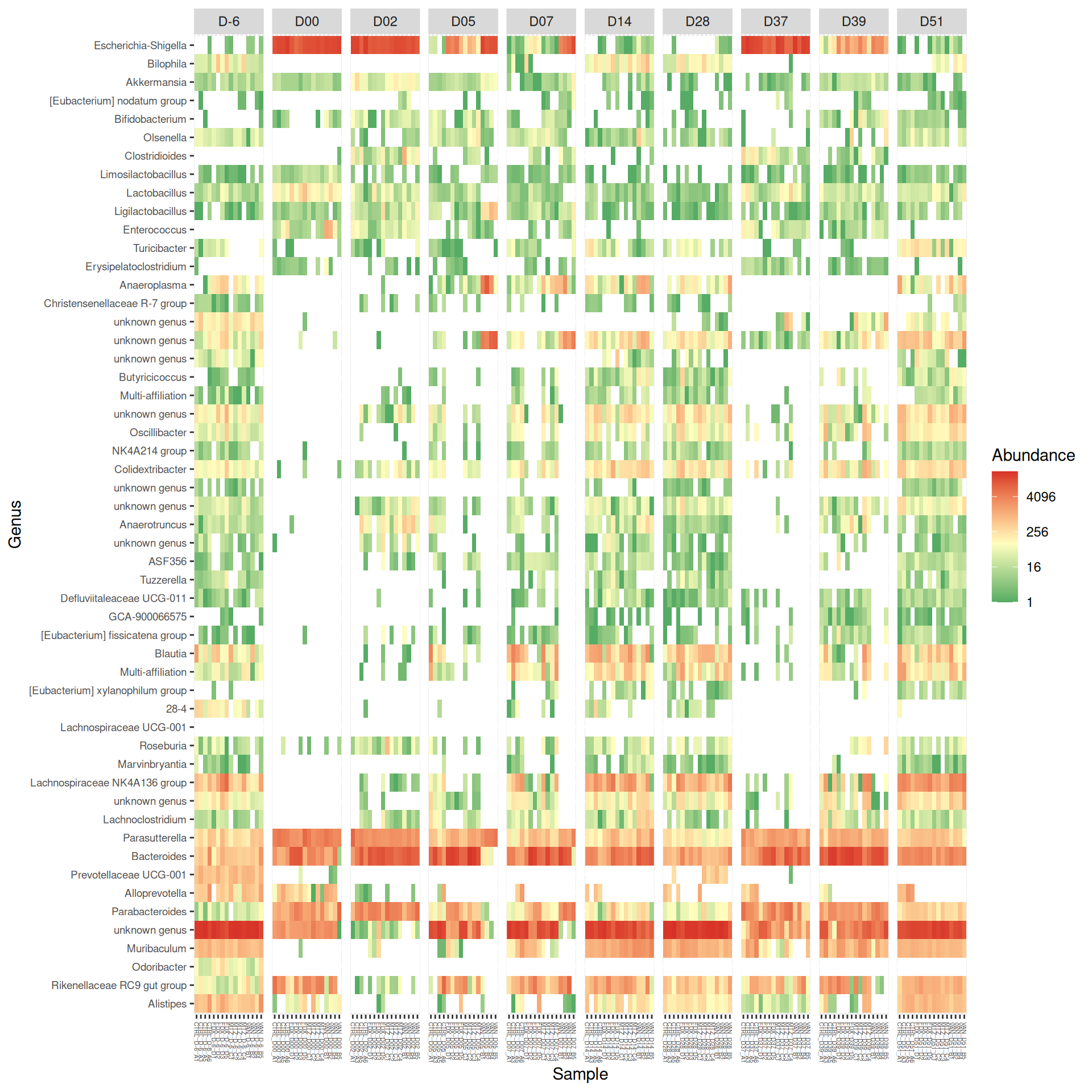
At Family and Genus taxonomic levels, we created heatmap plot using ordination methods to organize the rows.
# method = NULL if not ordinationp <- phyloseq::plot_heatmap(tax_glom(frogs_rare_withoutR, taxrank="Family"), method ="MDS",distance ="bray",sample.order="Label", # not ordination# taxa.order = "Family",taxa.label ="Family") +facet_grid(~ DAY, scales ="free_x", space ="free_x") +scale_fill_gradient2(low ="#1a9850", mid ="#ffffbf", high ="#d73027",na.value ="white", trans = scales::log_trans(4),midpoint =log(100, base =4))p
Show the code
p <- phyloseq::plot_heatmap(tax_glom(frogs_rare_withoutR, taxrank="Genus"), distance ="bray", method ="MDS",sample.order="Label", # not ordination# taxa.order = "Family",taxa.label="Genus") +facet_grid(~ DAY, scales ="free_x", space ="free_x") +scale_fill_gradient2(low ="#1a9850", mid ="#ffffbf", high ="#d73027",na.value ="white", trans = scales::log_trans(4),midpoint =log(100, base =4))p
Important
As expected many bacteria disappeared at D00 due to antiobitics. Clostridoides was absent at D-6, D00, D28 and D51. It was present at D02 and D39, and partially present during the evolution of the infection depending on the GROUP treatment. Abundance profiles appeared fairly similar similar at D-6, D00, D28 and D51. We observed differences for Bifidobacterium, 28-4, Oscillibacter, and Prevotellaceae UCG-001. The effect of the GROUP treatment is observed at D02 and renforced until D14 on the microbiota composition. To pinpoint a few bacteria that differ at family level (see heatmap): desulfovibrionaceae, Rikenellaceae, Enterobacteriaceae, Lachnospiraceae and many others. These differences can be observed at genus level to obtain more precise information (see heatmap).
Differential abundance analysis (without R samples)
We performed differential analysis from frogs object without rarefaction excluding re-infection R.
Show the code
# from Mahendra's functions# useful functions to perform a differential abundance analysis (daa)# filter taxa all zeros in all samples and # keep taxa with counts > 10 in at least the number of replicates - possibility to choosemy_filter_phyloseq <-function(physeq, nreplicates =2) { ii <- phyloseq::genefilter_sample(physeq, function(x) x >10, nreplicates) phyloseq::prune_taxa(ii, physeq)}# realise differential abundance results (daa) for the contrast# Note to specify a contrast as a listmy_extract_results <-function(deseq, test ="Wald", contrast) { DESeq2::results(deseq, test = test, tidy =TRUE, contrast = contrast) %>% dplyr::rename(ASV = row) %>%# dplyr::filter(padj <= 0.05) %>% dplyr::arrange(log2FoldChange)}# formatting the daa result by adding ASV informations into daa objectmy_format_results <-function(data, physeq) {tax_table(physeq)@.Data %>%as_tibble() %>%mutate(ASV =rownames(tax_table(physeq)@.Data)) %>% dplyr::right_join(., data, by ="ASV") %>%mutate(ASV =factor(ASV, levels = data$ASV))}# combine my_extract_results and my_format_results into an unique function# realise differential abundance results (daa) for the contrast# Note to specify a contrast as a listmy_daa_results <-function(deseq, test ="Wald", physeq, contrast) {# provide differential abundance results (daa) for the contrast# sort by log2FoldChange daa <- DESeq2::results(deseq, test = test, tidy =TRUE, contrast = contrast) %>% dplyr::rename(ASV = row) %>% dplyr::filter(padj <=0.05) # add ASV informations into daa object daa_new <-tax_table(physeq)@.Data %>%as_tibble() %>%mutate(ASV =rownames(tax_table(physeq)@.Data)) %>% dplyr::right_join(., daa, by ="ASV") %>%mutate(ASV =factor(ASV, levels = daa$ASV)) %>% dplyr::arrange(log2FoldChange)return(daa_new)}
phyloseq-class experiment-level object
otu_table()   OTU Table:         [ 52 taxa and 160 samples ]
sample_data() Sample Data:       [ 160 samples by 7 sample variables ]
tax_table()   Taxonomy Table:    [ 52 taxa by 7 taxonomic ranks ]
phy_tree()    Phylogenetic Tree: [ 52 tips and 51 internal nodes ]
Important
The differential abundance analysis (DAA) is based on a Generalized Linear Model (GLM) to take into account the distribution of count-type data (non-normality of the data) and over-dispersion. The regression coefficients of the factors are estimated in the model and Wald test was used to identify DAA ASV’s in a defined contrast.
Using DESeq2 R package, the GLM model [1] was fitted with GROUP treatment and DAY factors and the interaction. A Benjamini-Hochberg false discovery rate (FDR) correction [2] was applied on pvalues.
Show the code
# do not rarefy for differential analysiscds_2 <- phyloseq::phyloseq_to_deseq2(frogs_withoutR,~ GROUP*DAY)rowData(cds_2) <-tax_table(frogs_withoutR)# cds is a summarized experiment object SE# experimental design# colData(cds_2)# abundances# assays(cds_2)$counts# fit Negative Binomial GLM modeldds_2 <- DESeq2::DESeq(cds_2, sfType ="poscounts", fitType='local')dds_2_coeff <- DESeq2::resultsNames(dds_2)# identical results#res <- results(dds_2, contrast=c("GROUP", "FDX", "CTRL"))#res <- results(dds_2, name = "GROUP_FDX_vs_CTRL")#DESeq2::results(dds_2, test = "Wald", tidy = TRUE, contrast = c("GROUP", "FDX", "CTRL"))
Identify DAA between DAY
With this model, we performed differential analysis between consecutive days and eubiose days (D-6, D28, D51). See results at the end of this report.
Show the code
# define interesting contrastscontrast_DAY <-list("DAY_D00_vs_D-6"=c("DAY", "D00", "D-6"), "DAY_D02_vs_D00"=c("DAY", "D02", "D00"),"DAY_D05_vs_D02"=c("DAY", "D05", "D02"),"DAY_D07_vs_D05"=c("DAY", "D07", "D05"),"DAY_D14_vs_D07"=c("DAY", "D14", "D07"),"DAY_D28_vs_D14"=c("DAY", "D28", "D14"),"DAY_D37_vs_D28"=c("DAY", "D37", "D28"),"DAY_D39_vs_D37"=c("DAY", "D39", "D37"),"DAY_D51_vs_D39"=c("DAY", "D51", "D39"),"DAY_D28_vs_D-6"=c("DAY", "D28", "D-6"),"DAY_D51_vs_D28"=c("DAY", "D51", "D28") )#results#res <- results(dds_2, contrast=c("DAY", "D05", "D00"))# #extract result for a fixed contrast# daa_deseq2 <- my_extract_results(dds_2, contrast = contrast_DAY[[1]])# #format dda result for a fixed contrast# daa_res <- my_format_results(data = daa_deseq2, physeq = frogs_withoutR)# combine the previous functions# realize a differential abubdance analyses (dda) for a list of contrasts# format dda: adding ASV informations and sorting by log2FoldChangedaa_deseq2_DAY <- contrast_DAY |>map(\(x) my_daa_results(dds_2, test ="Wald", physeq = frogs_withoutR, contrast = x))
This is the number of differential abundance ASV obtained between the DAY.
Show the code
# number of ASV daa for each tested contrastdaa_deseq2_DAY |>map_df(nrow) |>t() |>kbl(col.names =c("Nb of diff. abundant ASV at Genus levels")) |>kable_styling() |>scroll_box(width ="60%", height ="200px")
Nb of diff. abundant ASV at Genus levels
DAY_D00_vs_D-6
41
DAY_D02_vs_D00
28
DAY_D05_vs_D02
23
DAY_D07_vs_D05
2
DAY_D14_vs_D07
2
DAY_D28_vs_D14
1
DAY_D37_vs_D28
32
DAY_D39_vs_D37
22
DAY_D51_vs_D39
16
DAY_D28_vs_D-6
1
DAY_D51_vs_D28
3
Identify DAA between GROUP
With this model, we performed differential analysis between the GROUP treatments. See results at the end of this report.
Show the code
# identical results#res <- results(dds_2, contrast=c("GROUP", "FDX", "CTRL"))#res <- results(dds_2, name = "GROUP_FDX_vs_CTRL")#DESeq2::results(dds_2, test = "Wald", tidy = TRUE, contrast = c("GROUP", "FDX", "CTRL"))# define interesting contrastscontrast_GROUP <-list("GROUP_FDX_vs_CTRL"=c("GROUP", "FDX", "CTRL"),"GROUP_MTZ_vs_CTRL"=c("GROUP", "MTZ", "CTRL"),"GROUP_VAN_vs_CTRL"=c("GROUP", "VAN", "CTRL"),"GROUP_VAN_vs_FDX"=c("GROUP", "VAN", "FDX"),"GROUP_VAN_vs_MTZ"=c("GROUP", "VAN", "MTZ"),"GROUP_FDX_vs_MTZ"=c("GROUP", "FDX", "MTZ") )# #extract result for a fixed contrast# daa_deseq2 <- my_extract_results(dds_2, contrast = contrast_GROUP[[1]])# #format dda result for a fixed contrast# daa_res <- my_format_results(data = daa_deseq2, physeq = frogs_withoutR)# combine the previous functions# realize a differential abubdance analyses (dda) for a list of contrasts# format dda: adding ASV informations and sorting by log2FoldChangedaa_deseq2_GROUP <- contrast_GROUP |>map(\(x) my_daa_results(dds_2, test ="Wald", physeq = frogs_withoutR, contrast = x))
This is the number of differential abundance ASV obtained between the GROUP treatments.
Show the code
# number of ASV daa for each tested contrastdaa_deseq2_GROUP |>map_df(nrow) |>t() |>kbl(col.names =c("Nb of diff. abundant ASV at Genus levels")) |>kable_styling() |>scroll_box(width ="60%", height ="200px")
Nb of diff. abundant ASV at Genus levels
GROUP_FDX_vs_CTRL
0
GROUP_MTZ_vs_CTRL
1
GROUP_VAN_vs_CTRL
0
GROUP_VAN_vs_FDX
0
GROUP_VAN_vs_MTZ
1
GROUP_FDX_vs_MTZ
1
Identify DAA between D05, D07, D14 Days
Important
The differential abundance analysis (DAA) is based on a Generalized Linear Model (GLM) to take into account the distribution of count-type data (non-normality of the data) and over-dispersion. The regression coefficients of the factors are estimated in the model and Wald test was used to identify DAA ASV’s in a defined contrast.
Using DESeq2 R package, the GLM model [1] was fitted with one factor combining the levels of GROUP treatment and DAY factors. A Benjamini-Hochberg false discovery rate (FDR) correction [2] was applied on pvalues.
Show the code
# do not rarefy# at defined level taxrank# filtering low abundance: less 10 in at least nreplicates# subset eubiose samplescds <- phyloseq::phyloseq_to_deseq2(frogs_withoutR,~0+ GROUPJ)rowData(cds) <-tax_table(frogs_withoutR)# cds is a summarized experiment object SE# experimental design# colData(cds)# abundances# assays(cds)$counts# fit Negative Binomial GLM modeldds <- DESeq2::DESeq(cds, sfType ="poscounts", fitType='local')dds_coeff <- DESeq2::resultsNames(dds)# # at fixed DAY between treatmentcontrast_D05_D07_D14 <-list("D05_FDXvsCTRL"=c("GROUPJFDX_D05", "GROUPJCTRL_D05"),"D05_MTZvsCTRL"=c("GROUPJMTZ_D05", "GROUPJCTRL_D05"),"D05_VANvsCTRL"=c("GROUPJVAN_D05", "GROUPJCTRL_D05"),"D05_FDXvsVAN"=c("GROUPJFDX_D05", "GROUPJVAN_D05"),"D05_MTZvsVAN"=c("GROUPJMTZ_D05", "GROUPJVAN_D05"),"D05_FDXvsMTZ"=c("GROUPJFDX_D05", "GROUPJMTZ_D05"),"D07_FDXvsCTRL"=c("GROUPJFDX_D07", "GROUPJCTRL_D07"),"D07_MTZvsCTRL"=c("GROUPJMTZ_D07", "GROUPJCTRL_D07"),"D07_VANvsCTRL"=c("GROUPJVAN_D07", "GROUPJCTRL_D07"),"D07_FDXvsVAN"=c("GROUPJFDX_D07", "GROUPJVAN_D07"),"D07_MTZvsVAN"=c("GROUPJMTZ_D07", "GROUPJVAN_D07"),"D07_FDXvsMTZ"=c("GROUPJFDX_D07", "GROUPJMTZ_D07"),"D14_FDXvsCTRL"=c("GROUPJFDX_D14", "GROUPJCTRL_D14"),"D14_MTZvsCTRL"=c("GROUPJMTZ_D14", "GROUPJCTRL_D14"),"D14_VANvsCTRL"=c("GROUPJVAN_D14", "GROUPJCTRL_D14"),"D14_FDXvsVAN"=c("GROUPJFDX_D14", "GROUPJVAN_D14"),"D14_MTZvsVAN"=c("GROUPJMTZ_D14", "GROUPJVAN_D14"),"D14_FDXvsMTZ"=c("GROUPJFDX_D14", "GROUPJMTZ_D14") )# combine the previous functions# realize a differential abubdance analyses (dda) for a list of contrasts# format dda: adding ASV informations and sorting by log2FoldChangedaa_deseq2_D05_D07_D14 <- contrast_D05_D07_D14 |>map(\(x) my_daa_results(dds, test ="Wald", physeq = frogs_withoutR, contrast =list(x))) #daa_deseq2_D05_D07_D14
This is the number of differential abundance ASV obtained for each tested contrast: pairwise contrast between the levels of GROUP treatment at D05, D07, D14 values of DAY.
Show the code
# number of ASV daa for each tested contrastdaa_deseq2_D05_D07_D14 |>map_df(nrow) |>t() |>kbl(col.names =c("Nb of diff. abundant ASV at Genus levels")) |>kable_styling() |>scroll_box(width ="60%", height ="200px")
Nb of diff. abundant ASV at Genus levels
D05_FDXvsCTRL
36
D05_MTZvsCTRL
39
D05_VANvsCTRL
34
D05_FDXvsVAN
35
D05_MTZvsVAN
32
D05_FDXvsMTZ
35
D07_FDXvsCTRL
38
D07_MTZvsCTRL
40
D07_VANvsCTRL
35
D07_FDXvsVAN
43
D07_MTZvsVAN
35
D07_FDXvsMTZ
36
D14_FDXvsCTRL
44
D14_MTZvsCTRL
41
D14_VANvsCTRL
42
D14_FDXvsVAN
44
D14_MTZvsVAN
43
D14_FDXvsMTZ
42
heatmap
Heatmap [3] allow visual comparison of abundances between taxa in different samples. To do this, abundances should be normalized to remove compositionality bias between samples.
Show the code
# transformation clr # scaled transformation on the rows (subtracting mean and dividing by var)frogs_clr_Z <- frogs_withoutRtmp <- vegan::decostand(otu_table(frogs_withoutR), "clr", pseudocount=1, log =exp(1), MARGIN =2)tmp <- vegan::decostand(tmp, "standardize", MARGIN =1)# replace abundances counts by clr + Z's transformationotu_table(frogs_clr_Z) <-otu_table(tmp, taxa_are_rows=TRUE)#frogs_clr_Z <- frogs_clr_Z %>% microViz::ps_arrange(DAY, GROUP)frogs_clr_Z
phyloseq-class experiment-level object
otu_table()   OTU Table:         [ 52 taxa and 160 samples ]
sample_data() Sample Data:       [ 160 samples by 7 sample variables ]
tax_table()   Taxonomy Table:    [ 52 taxa by 7 taxonomic ranks ]
phy_tree()    Phylogenetic Tree: [ 52 tips and 51 internal nodes ]
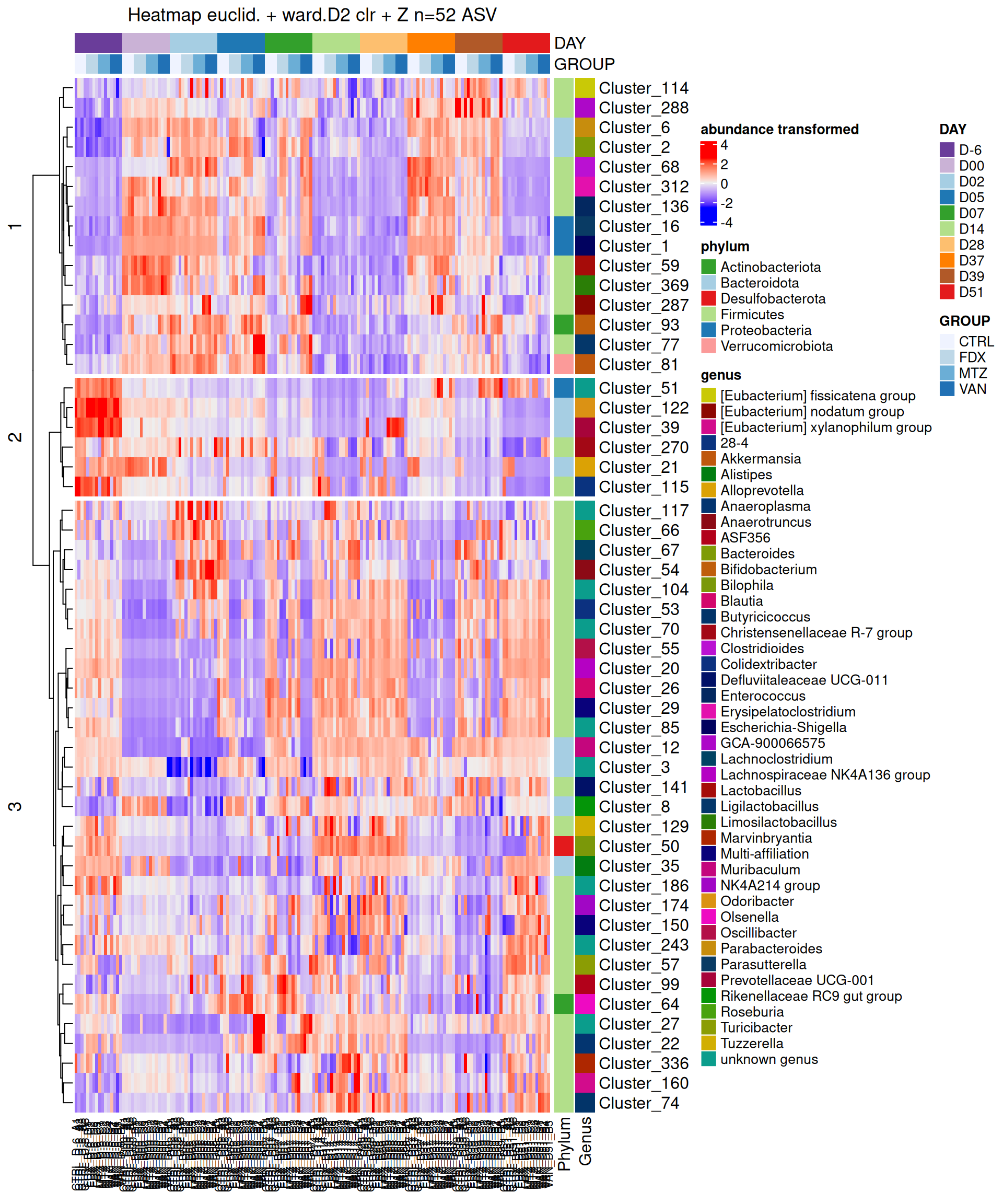
A hierarchical clustering followed by a heatmap plot [3] were performed on all ASV with abundances aggregated at Genus taxa rank, with ComplexHeatmap R package. We do not used results from differential analysis.
Here, the centered log-ratio (CLR) transformation [4] were performed: abundances were divided by the geometric mean of the read counts of all taxa within a sample and then the log fold changes in this ratio is applied. CLR-transformed data were standardized (taxa have zero mean and unit variance) to allow the comparison between taxa.
Hierarchical clustering was performed on rows in two steps: 1/ calculate the euclidean distance and 2/ apply a clustering method with the Ward’s distance. The dendrogram was cut to obtain groups of taxa with similar behaviour. Note that the number of clusters was chosen arbitrarily.
Note that the samples were not clustered but ordered by DAY and GROUP.
Description
Excel file containing the results of alpha diversity tests for eubiose samples with rarefaction based on the complete study
Excel file containing the results of differential abundance analysis between consecutive days and eubiose days
Excel file containing the results of differential abundance analysis between GROUP treatment
Excel file containing the results of differential abundance analysis between GROUP treatment at D05, D07, D14 days
2. Benjamini Y, Hochberg Y. Controlling the false discovery rate: A practical and powerful approach to multiple testing. Journal of the Royal Statistical Society Series B (Methodological). 1995;57:289–300. http://www.jstor.org/stable/2346101.
3. Gu Z, Eils R, Schlesner M. Complex heatmaps reveal patterns and correlations in multidimensional genomic data. Bioinformatics. 2016;32:2847–9. doi:10.1093/bioinformatics/btw313.
4. Aitchison J. The statistical analysis of compositional data, monographs on statistics and applied probability (chapman & hall, london. In: Reprinted in 2003 with additional material by the blackburn press. Frontiers Media SA; 1986. p. 416–p.
Reuse
This document will not be accessible without prior agreement of the partners
A work by Migale Bioinformatics Facility
Université Paris-Saclay, INRAE, MaIAGE, 78350, Jouy-en-Josas, France
Université Paris-Saclay, INRAE, BioinfOmics, MIGALE bioinformatics facility, 78350, Jouy-en-Josas, France
Source Code
---title: "ICD"search: falsenavbar: falsesubtitle: "Accompaniement of Anaïs Brosse in her analyses"author: - name: Olivier Rué orcid: 0000-0003-1689-0557 email: olivier.rue@inrae.fr affiliations: - name: Migale bioinformatics facility adress: Domaine de Vilvert city: Jouy-en-Josas state: France - name: Christelle Hennequet-Antier orcid: 0000-0001-5836-2803 email: christelle.hennequet-antier@inrae.fr affiliations: - name: Migale bioinformatics facility adress: Domaine de Vilvert city: Jouy-en-Josas state: Francedate: "2023-07-05"date-modified: todayimage: "images/preview.jpg"reader-mode: falsefig-cap-location: bottomtbl-cap-location: toplicense: "This document will not be accessible without prior agreement of the partners"format: html: embed-resources: false toc: true code-fold: true code-summary: "Show the code" code-tools: true toc-location: right page-layout: article code-overflow: wrap---```{r setup, include=FALSE}knitr::opts_chunk$set(eval=TRUE, echo =TRUE, cache = FALSE, message = FALSE, warning = FALSE, cache.lazy = FALSE, fig.height = 3.5, fig.width = 10)``````{r}#| label: load-packages#library(DT)library(tidyverse)library(kableExtra)library(phyloseq)library(phyloseq.extended)library(data.table)library(InraeThemes)library(readr) #read_delimlibrary(ggplot2) # graphicslibrary(microbiome) # for boxplot_alpha functionlibrary(mia) # microbiome analysis with SummarizedExperiment and TreeSummarizedExperimentlibrary(emmeans) #post hoc testslibrary(reactable) #table formatting and stylinglibrary(reactablefmtr) #table formatting and stylinglibrary(openxlsx) #save results to excel sheetslibrary(metacoder) # differential abundancelibrary(ggtree) # visualizationlibrary(ggtreeExtra) # visualizationlibrary(ComplexHeatmap) # produce heatmaplibrary(microViz) # analysis and visualization of microbiome sequencing data```<!-- ```{r datatable global options, echo=FALSE, eval=TRUE} --><!-- options(DT.options = list(pageLength = 10, --><!-- scrollX = TRUE, --><!-- language = list(search = 'Filter:'), --><!-- dom = 'lftipB', --><!-- buttons = c('copy', 'csv', 'excel'))) --><!-- ``` -->{{< include /resources/_includes/_intro_note.qmd >}}# Aim of the projectInfluence of treatment antibiotics in a murine model of infection with *Clostridium difficile* (ICD). Injection of *C. difficile* were performed at `J00` and `J37`.- Différencier les groupes ctrl et traités aux antibiotiques (VAN, MTZ, FDX, R = réinfections multiples), et comparer les cinétiques entre les groupes. Les échantillons contrôle sont infectés mais pas traités aux antibiotiques.- Etudier les cinétiques au sein des traitements (CTRL, VAN, MTZ, FDX, R). Est-ce qu’il y a un retour à J-6 ? Clairance de la bactérie (zéro dans les fécès, attention biofilm et sporulation peuvent encore existés)- Eubiose : comparer J-6, J28, J51. ## Partners* Olivier Rué - Migale bioinformatics facility - BioInfomics - INRAE* Christelle Hennequet-Antier - Migale bioinformatics facility - BioInfomics - INRAE* Mahendra Mariadassou - Migale bioinformatics facility - BioInfomics - INRAE* Anaïs Brosse - MICALIS - INRAE# Data management{{< include /resources/_includes/_data_management.qmd >}}# Analyses## Experiment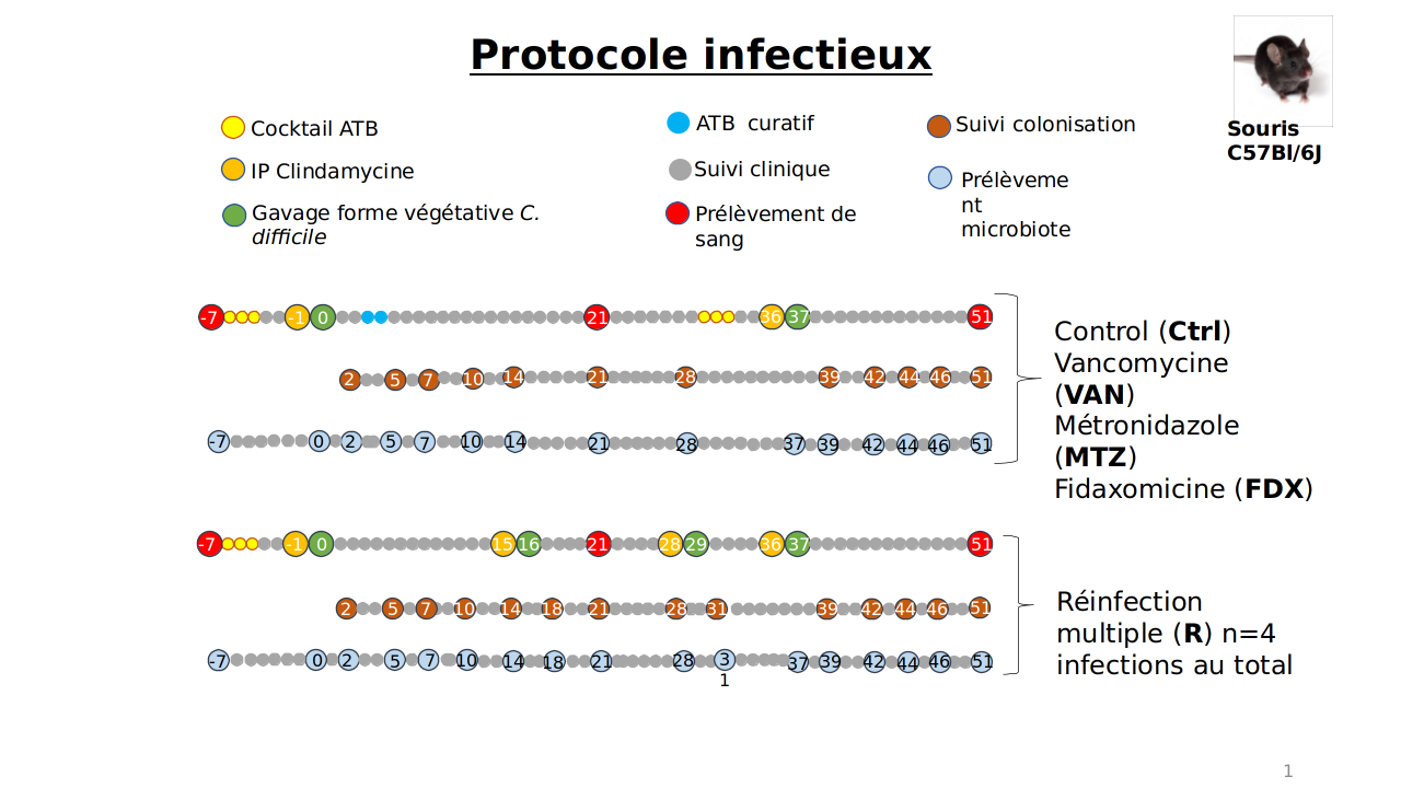{fig-align="center"}# Phyloseq rarefied data with all samples ```{r}#| label: load-datafrogs <-readRDS(file ="../html/frogs.rds")```For having the same sampling depth for all samples, we rarefy them before exploring the diversity.```{r}#| label: frogs_rarefrogs_rare <- phyloseq::rarefy_even_depth(frogs, rngseed =123, replace =TRUE)``````{r}#| echo: false#| eval: falsephyloseq::plot_bar(frogs_rare, x="REPLICAT", fill="Phylum") +facet_grid(GROUP~DAY, scales="free_x")```# study on subset excluding R treatment::: {.callout-important}Note that the rarefaction was performed on all samples from the complete study. We extracted samples of interest from the `frogs_rare` phyloseq object to calculate alpha diversity. Alpha diversity is calculated within sample and do not change with the previous analyses on the complete study.:::```{r}frogs_rare_withoutR <-subset_samples(frogs_rare, GROUP !="R")```## Taxonomic composition After rarefaction, let's have a look at the Phylum and genus levels composition with two types of plot.We explore composition using all samples.::: {.panel-tabset}### All By GROUP```{r}#| fig-width: 20#| class: superbigimagephyloseq.extended::plot_composition(frogs_rare_withoutR, NULL, NULL, "Phylum") +facet_grid(~ GROUP + DAY, scales ="free_x", space ="free_x") +scale_fill_brewer(palette ="Paired") +theme(axis.text.x =element_text(size =6, hjust =1)) +theme(legend.position="top")```### All By grid at phylum level```{r}#| fig-height: 10phyloseq.extended::plot_composition(frogs_rare_withoutR, NULL, NULL, "Phylum", x ="SOURIS") +facet_grid(rows =vars(DAY), cols =vars(GROUP), scales ="free_x", space ="free_x") +scale_fill_brewer(palette ="Paired") +theme(axis.text.x =element_text(size =6, hjust =1)) +theme(legend.position="top")```### All By grid at family level```{r}#| fig-height: 10phyloseq.extended::plot_composition(frogs_rare_withoutR, NULL, NULL, "Family", x ="SOURIS") +facet_grid(rows =vars(DAY), cols =vars(GROUP), scales ="free_x", space ="free_x") +scale_fill_brewer(palette ="Paired") +theme(axis.text.x =element_text(size =6, hjust =1)) +theme(legend.position="top")```::: ## Alpha-Diversity on subset excluding R treatmentBoxplot of alpha-diversity facetting by `DAY`.::: {.panel-tabset}### All```{r}#| fig-height: 10# plot alpha diversity# measures = c("Observed", "Chao1", "Shannon", "Simpson", "InvSimpson")p <- phyloseq::plot_richness(physeq = frogs_rare_withoutR, x ="DAY", color="GROUP", title ="Alpha diversity graphics", measures =c("Observed", "Shannon"), nrow=5) +geom_jitter() +scale_fill_brewer(palette ="Paired") +theme(axis.text.x =element_text(size =6, angle =45, hjust =1)) +theme(legend.position="top")p```### Observed```{r}#| fig-height: 10# plot alpha diversity p.alphadiversity <- microbiome::boxplot_alpha(frogs_rare_withoutR, index ="Observed",x_var ="GROUP")p.alphadiversity +facet_grid(cols =vars(DAY), scales ="free_x", space ="free_x") +scale_fill_brewer(palette ="Paired") +theme(axis.text.x =element_text(size =6, angle =45, hjust =1)) +theme(legend.position="top")```<!-- ### Chao1 --><!-- ```{r} --><!-- #| fig-height: 10 --><!-- # plot alpha diversity --><!-- p.alphadiversity <- microbiome::boxplot_alpha(frogs_rare_withoutR, --><!-- index = "Chao1", --><!-- x_var = "GROUP") --><!-- p.alphadiversity + --><!-- facet_grid(cols = vars(DAY), scales = "free_x", space = "free_x") + --><!-- scale_fill_brewer(palette = "Paired") + --><!-- theme(axis.text.x = element_text(size = 6, angle = 45, hjust = 1)) + --><!-- theme(legend.position="top") --><!-- ``` -->### Shannon```{r}#| fig-height: 10# plot alpha diversity p.alphadiversity <- microbiome::boxplot_alpha(frogs_rare_withoutR, index ="Shannon",x_var ="GROUP")p.alphadiversity +facet_grid(cols =vars(DAY), scales ="free_x", space ="free_x") +scale_fill_brewer(palette ="Paired") +theme(axis.text.x =element_text(size =6, angle =45, hjust =1)) +theme(legend.position="top")```<!-- ### Simpson --><!-- ```{r} --><!-- #| fig-height: 10 --><!-- # plot alpha diversity --><!-- p.alphadiversity <- microbiome::boxplot_alpha(frogs_rare_withoutR, --><!-- index = "Simpson", --><!-- x_var = "GROUP") --><!-- p.alphadiversity + --><!-- facet_grid(cols = vars(DAY), scales = "free_x", space = "free_x") + --><!-- scale_fill_brewer(palette = "Paired") + --><!-- theme(axis.text.x = element_text(size = 6, angle = 45, hjust = 1)) + --><!-- theme(legend.position="top") --><!-- ``` -->:::<!-- ::: {.callout-important} --><!-- We observed that the alpha-diversity is mainly determined by `DAY` rather than `GROUP`. For each sample, the observed index measures the richness in the sample i.e. the total number of species in the community. Richness was highest in samples from `J-6` and `J51`, and also `J28` with more variability. It decreased on `J00`, and `J37` on days of infection, and increased between infection dates. The other indices do not provide any additional information, as the trajectories are consistent with infection dates. --><!-- ::: -->## Alpha-diversity - statistical testsWe calculated the alpha-diversity indices and combined them with covariates from experimental design.```{r}div_data <-cbind(estimate_richness(frogs_rare_withoutR), ## diversity indicessample_data(frogs_rare_withoutR) ## covariates )```### Model ```{r}#model <- aov(Observed ~ DAY*GROUP, data = div_data)#anova(model)#coef(model)# produce parwise comparison test with Tukey's post-hoc correction #TukeyHSD(model, which ="DAY:GROUP")alphadiv.lm <-lm(Observed ~ DAY*GROUP, data = div_data)anova(alphadiv.lm)# interaction visualisationpar(mfrow =c(1,2))emmip(alphadiv.lm, GROUP ~ DAY, CIs =TRUE)emmip(alphadiv.lm, DAY ~ GROUP, CIs =TRUE)par(mfrow =c(1,1))#tests EMM <-emmeans(alphadiv.lm, ~ DAY*GROUP)# tests correction are performed within the variable# P value adjustment: tukey method for comparing a family of 12 estimatescomp1 <-pairs(EMM, simple ="DAY")# P value adjustment: tukey method for comparing a family of 5 estimates comp2 <-pairs(EMM, simple ="GROUP")``````{r}# P value adjustment: tukey method for comparing a family of 60 estimatesres_emm <-contrast(EMM, method ="revpairwise", by =NULL,enhance.levels =c("DAY", "GROUP"), adjust ="tukey")``````{r}#| echo: false# using openxlsx package to export resultsexcelsheets <-list(All = res_emm, compbyGROUP = comp1, compbyDAY = comp2)write.xlsx(excelsheets, file =paste0("./comparisons_alpha_diversity_rareAll_withoutR", ".xlsx"))```::: {.callout-important}Richness is significantly different by `DAY`, `GROUP` and the interaction `DAY:GROUP`. Pairwise tests between `DAY` and `GROUP` were performed with post hoc Tukey's test to determine which were significant. We observed differences between the `GROUP` treatments at D05, D07, D14 and also at D39 in other way.:::```{r}#| eval: true#| echo: false# https://glin.github.io/reactable/index.html# https://glin.github.io/reactable/articles/custom-filtering.html#table-search-methods# TO DO# - filter min p.value# - search contrast# color value pvalue on significance# remplir en gris lorsque p.value tukey est non signif# save# table from results of contrast# visualize estimate and p.valuecomp_table <-read.xlsx(xlsxFile ="./comparisons_alpha_diversity_rareAll_withoutR.xlsx", sheet =2)comp_table <- comp_table %>%na.omit() %>%select(GROUP, contrast, estimate, p.value) %>%mutate(estimate =round(estimate, digits=2)) reactable(comp_table,theme =nytimes(centered =TRUE),compact =TRUE,defaultSortOrder ='asc',defaultSorted =c('GROUP', 'contrast', 'p.value'),columns =list(GROUP =colDef(name ='By Family', minWidth =70,# searchable = TRUE,# searchMethod = ),contrast =colDef(name ='comparison', minWidth =70,# searchable = TRUE,# searchMethod = ),estimate =colDef(name ='estimate',minWidth =150,align ='center',cell =data_bars(data = comp_table,text_position ='outside-end',fill_color =c('#C40233','#127852'),number_fmt = scales::label_number(accuracy =0.01) ) ),p.value =colDef(name ="Tukey's p.value",minWidth =70,align ='center',filterable =TRUE ) ))``````{r}#| eval: true#| echo: false# https://glin.github.io/reactable/index.html# https://glin.github.io/reactable/articles/custom-filtering.html#table-search-methods# TO DO# - filter min p.value# - search contrast# color value pvalue on significance# remplir en gris lorsque p.value tukey est non signif# save# table from results of contrast# visualize estimate and p.valuecomp_table <-read.xlsx(xlsxFile ="./comparisons_alpha_diversity_rareAll_withoutR.xlsx", sheet =3)comp_table <- comp_table %>%na.omit() %>%select(DAY, contrast, estimate, p.value) %>%mutate(estimate =round(estimate, digits=2)) reactable(comp_table,theme =nytimes(centered =TRUE),compact =TRUE,defaultSortOrder ='asc',defaultSorted =c('DAY', 'contrast', 'p.value'),columns =list(DAY =colDef(name ='By Family', minWidth =70,# searchable = TRUE,# searchMethod = ),contrast =colDef(name ='comparison', minWidth =70,# searchable = TRUE,# searchMethod = ),estimate =colDef(name ='estimate',minWidth =150,align ='center',cell =data_bars(data = comp_table,text_position ='outside-end',fill_color =c('#C40233','#127852'),number_fmt = scales::label_number(accuracy =0.01) ) ),p.value =colDef(name ="Tukey's p.value",minWidth =70,align ='center',filterable =TRUE ) ))``````{r}#| eval: true#| echo: false# https://glin.github.io/reactable/index.html# https://glin.github.io/reactable/articles/custom-filtering.html#table-search-methods# TO DO# - filter min p.value# - search contrast# color value pvalue on significance# remplir en gris lorsque p.value tukey est non signif# save# # table from results of contrast# visualize estimate and p.valuecomp_table <-read.xlsx(xlsxFile ="./comparisons_alpha_diversity_rareAll_withoutR.xlsx", sheet =1)comp_table <- comp_table %>%na.omit() %>%select(contrast, estimate, p.value) %>%mutate(estimate =round(estimate, digits=2)) # comp_table <- comp_table %>%# na.omit() %>%# select(contrast, estimate, p.value) %>%# mutate(estimate = round(estimate, digits=2)) %>%# mutate(log10p.value = -log10(p.value)) %>%# mutate(signif = case_when(# p.value < 0.05 ~ '#C40233',# p.value >= 0.05 ~ 'gray'# )# )reactable(comp_table,theme =nytimes(centered =TRUE),compact =TRUE,defaultSortOrder ='asc',defaultSorted ='p.value',columns =list(contrast =colDef(name ='comparison', minWidth =150,# searchable = TRUE,# searchMethod = ),estimate =colDef(name ='estimate',minWidth =150,align ='center',cell =data_bars(data = comp_table,text_position ='outside-end',fill_color =c('#C40233','#127852'),number_fmt = scales::label_number(accuracy =0.01) ) ),p.value =colDef(name ="Tukey's p.value",minWidth =70,align ='center',filterable =TRUE ) ))```## Beta-diversity on subset excluding R treatmentThe dissimilarity between samples based on taxonomic composition is calculated with one of these Beta diversities: Bray-Curtis, Unweighted and weighted Unifrac, Jaccard index. The Jaccard index uses presence/absence information only whereas UniFrac integrates information from the phylogenetic tree.```{r}# use all samples from the complete study frogs_raredist.jac <- phyloseq::distance(frogs_rare, method ="cc")dist.bc <- phyloseq::distance(frogs_rare, method ="bray")dist.uf <- phyloseq::distance(frogs_rare, method ="unifrac")dist.wuf <- phyloseq::distance(frogs_rare, method ="wunifrac")distance_list <-list("Jaccard"= dist.jac,"Bray-Curtis"= dist.bc,"UniFrac"= dist.uf,"wUniFrac"= dist.wuf)``````{r}#| echo: true#| eval: true# Mahendra's function# used own color's palette and shapemy_plot2 <-function(variable1, variable2, physeq = mydata_rare, shapeval, colorpal) { .plot <-function(distance) { .distance <- distance_list[[distance]] %>%as.matrix() %>%`[`(sample_names(physeq), sample_names(physeq)) %>%as.dist() p <-plot_ordination(physeq,ordinate(physeq, method ="MDS", distance = .distance),color = variable1, shape = variable2) +scale_shape_manual(values = shapeval) +scale_color_manual(name = colorpal$name,labels = colorpal$labels,values = colorpal$values ) +theme(legend.position ="none") +ggtitle(distance)# print(p) } plots <-lapply(names(distance_list), .plot) legend <- cowplot::get_legend(plots[[1]] +theme(legend.position ="bottom")) pgrid <- cowplot::plot_grid(plotlist = plots) cowplot::plot_grid(pgrid, legend, ncol =1, rel_heights =c(1, .1))}``````{r pcoa_with_arrows}#| echo: true#| eval: true# Mahendra's function# used own color's palette and shapemy_pcoa_with_arrows2 <- function(physeq = mydata_rare, variable1, variable2, shapeval, colorpal) { # select samples of interest where all samples were used to calculate the distances between samples # dist.jac is previously calculated with all samples of the study #dist.c <- phyloseq::distance(physeq, "jaccard") #dist.c <- dist.jac %>% as.matrix() %>% `[`(sample_names(physeq), sample_names(physeq)) %>% as.dist() dist.c <- dist.bc %>% as.matrix() %>% `[`(sample_names(physeq), sample_names(physeq)) %>% as.dist() ord.c <- ordinate(physeq, "MDS", dist.c) p <- plot_ordination(physeq, ord.c) # ## Build arrow data plot_data <- p$data arrow_data <- plot_data %>% group_by(pick({{variable2}}, {{variable1}})) %>% arrange({{variable1}}) %>% mutate(xend = Axis.1, xstart = lag(xend), yend = Axis.2, ystart = lag(yend) ) ## Plot with arrows p + aes(shape = .data[[ variable2 ]], color = .data[[ variable1 ]]) + scale_shape_manual(values = shapeval) + scale_color_manual(name = colorpal$name, labels = colorpal$labels, values = colorpal$values) + theme_bw() + geom_segment(data = arrow_data, aes(x = xstart, y = ystart, xend = xend, yend = yend), size = 0.8, linetype = "3131", arrow = arrow(length=unit(0.1,"inches")), show.legend = FALSE) + geom_point(size = 3) + theme(legend.position = "bottom")}``````{r}#| fig-height: 6#| warning: false# MDS plot for samples of interests # from distance calculated with all samples of the complete study# used https://colorbrewer2.org/#type=qualitative&scheme=Paired&n=12Jour_pal <-list(name ="DAY",labels =c("D-6", "D00", "D02", "D05", "D07", "D14", "D28", "D37", "D39", "D51"),values =c("#6a3d9a", "#cab2d6", "#a6cee3", "#1f78b4", "#33a02c", "#b2df8a", "#fdbf6f", "#ff7f00", "#b15928", "#e31a1c"))GROUP_shape <-list(values =c(1, 15, 16, 17))my_plot2(variable1 ="DAY",variable2 ="GROUP",physeq = frogs_rare_withoutR,shapeval = GROUP_shape$values,colorpal = Jour_pal )```The percentage of variance explained on the first two axes of the MDS plot is 59.5% (=43.8 + 15.7) and 46.5% (=38 +8.5) for the Bray-Curtis and Jaccard distances, respectively.We use the Bray-Curtis's distance and show MDS trajectories of the communities intra conditions. ```{r}#| fig-height: 6# MDS plot for samples of interests # from distance calculated with all samples of the complete study# used https://colorbrewer2.org/#type=qualitative&scheme=Paired&n=12Jour_pal <-list(name ="DAY",labels =c("D-6", "D00", "D02", "D05", "D07", "D14", "D28", "D37", "D39", "D51"),values =c("#6a3d9a", "#cab2d6", "#a6cee3", "#1f78b4", "#33a02c", "#b2df8a", "#fdbf6f", "#ff7f00", "#b15928", "#e31a1c"))GROUP_shape <-list(values =c(1, 15, 16, 17))p <-my_pcoa_with_arrows2(variable1 ="DAY",variable2 ="GROUP",physeq = frogs_rare_withoutR,shapeval = GROUP_shape$values,colorpal = Jour_pal)p```::: {.callout-important}The multidimensional scaling (MDS / PCoA) showed that the samples were distributed according to the variable `DAY` and the evolution of the infection on the two first axes. The samples from `D-6`, `D28` and `D51` are close to each other, and opposite to those from `D00`, `D02` and `D37` on the first axis. The microbiota composition depends on the `DAY` and `GROUP` treatment which is reflected by the variability on the two axes. The differences between the `GROUP` treatments are more visible at D05, D07, D14 and also at D39.:::## Beta-diversity - Tests```{r}#| warning: falsemetadata <-sample_data(frogs_rare_withoutR) %>%as("data.frame")# choose bray-curtisdist.c <- dist.bc %>%as.matrix() %>%`[`(sample_names(frogs_rare_withoutR), sample_names(frogs_rare_withoutR)) %>%as.dist()# dist.c <- dist.jac %>% as.matrix() %>% `[`(sample_names(frogs_rare_withoutR), sample_names(frogs_rare_withoutR)) %>% as.dist()model <- vegan::adonis2(dist.c ~ DAY*GROUP, data = metadata, permutations =9999)print(model)```::: {.callout-important}The change in microbiota composition measured by the `Bray-Curtis` Beta diversity is significantly different between `DAY`, `GROUP` and also between the levels of the interaction factor `DAY:GROUP` at 0.05 significance level. The influence of the factors differs between ecosystems.:::```{r}#| label: clustering_samplespar(mfrow=c(1,1))par(mar =c(3, 0, 2, 0), cex =0.7)phyloseq.extended::plot_clust(frogs_rare_withoutR, dist ="bray", method ="ward.D2", color ="DAY",title ="Clustering of samples (Bray-Curtis + Ward)")# phyloseq.extended::plot_clust(frogs_rare_withoutR, dist = "jaccard", method = "ward.D2", color = "DAY",# title = "Clustering of samples (Jaccard + Ward)")```::: {.callout-important}Hierarchical clustering based on the `Bray-Curtis` dissimilarity and the `Ward` aggregation criterion shows that sample composition is not entirely structured by `DAY`. Groups were formed according to the date of infection and the existing `DAY:GROUP` interaction. :::<!-- ```{r} --><!-- #| label: heatmap_ordination --><!-- #| fig-height: 10 --><!-- p <- plot_heatmap(frogs_rare, distance = "bray", taxa.label="Phylum") + --><!-- facet_grid(~ DAY, scales = "free_x", space = "free_x") + --><!-- scale_fill_gradient2(low = "#1a9850", mid = "#ffffbf", high = "#d73027", --><!-- na.value = "white", trans = scales::log_trans(4), --><!-- midpoint = log(100, base = 4)) --><!-- p --><!-- ``` -->At Family and Genus taxonomic levels, we created heatmap plot using ordination methods to organize the rows.::: {.panel-tabset}### Family```{r}#| label: heatmap_ordination_Family#| fig-height: 10# method = NULL if not ordinationp <- phyloseq::plot_heatmap(tax_glom(frogs_rare_withoutR, taxrank="Family"), method ="MDS",distance ="bray",sample.order="Label", # not ordination# taxa.order = "Family",taxa.label ="Family") +facet_grid(~ DAY, scales ="free_x", space ="free_x") +scale_fill_gradient2(low ="#1a9850", mid ="#ffffbf", high ="#d73027",na.value ="white", trans = scales::log_trans(4),midpoint =log(100, base =4))p```### Genus```{r}#| label: heatmap_ordination_Genus#| fig-height: 10p <- phyloseq::plot_heatmap(tax_glom(frogs_rare_withoutR, taxrank="Genus"), distance ="bray", method ="MDS",sample.order="Label", # not ordination# taxa.order = "Family",taxa.label="Genus") +facet_grid(~ DAY, scales ="free_x", space ="free_x") +scale_fill_gradient2(low ="#1a9850", mid ="#ffffbf", high ="#d73027",na.value ="white", trans = scales::log_trans(4),midpoint =log(100, base =4))p```:::::: {.callout-important}As expected many bacteria disappeared at `D00` due to antiobitics. *Clostridoides* was absent at `D-6`, `D00`, `D28` and `D51`. It was present at `D02` and `D39`, and partially present during the evolution of the infection depending on the `GROUP` treatment. Abundance profiles appeared fairly similar similar at `D-6`, `D00`, `D28` and `D51`. We observed differences for *Bifidobacterium*, *28-4*, *Oscillibacter*, and *Prevotellaceae UCG-001*. The effect of the `GROUP` treatment is observed at `D02` and renforced until `D14` on the microbiota composition. To pinpoint a few bacteria that differ at family level (see heatmap): desulfovibrionaceae, Rikenellaceae, Enterobacteriaceae, Lachnospiraceae and many others. These differences can be observed at genus level to obtain more precise information (see heatmap). :::# Differential abundance analysis (without R samples)We performed differential analysis from `frogs` object without rarefaction excluding re-infection `R`. ```{r}#| label: my_functions_DESeq2#| echo: true#| eval: true# from Mahendra's functions# useful functions to perform a differential abundance analysis (daa)# filter taxa all zeros in all samples and # keep taxa with counts > 10 in at least the number of replicates - possibility to choosemy_filter_phyloseq <-function(physeq, nreplicates =2) { ii <- phyloseq::genefilter_sample(physeq, function(x) x >10, nreplicates) phyloseq::prune_taxa(ii, physeq)}# realise differential abundance results (daa) for the contrast# Note to specify a contrast as a listmy_extract_results <-function(deseq, test ="Wald", contrast) { DESeq2::results(deseq, test = test, tidy =TRUE, contrast = contrast) %>% dplyr::rename(ASV = row) %>%# dplyr::filter(padj <= 0.05) %>% dplyr::arrange(log2FoldChange)}# formatting the daa result by adding ASV informations into daa objectmy_format_results <-function(data, physeq) {tax_table(physeq)@.Data %>%as_tibble() %>%mutate(ASV =rownames(tax_table(physeq)@.Data)) %>% dplyr::right_join(., data, by ="ASV") %>%mutate(ASV =factor(ASV, levels = data$ASV))}# combine my_extract_results and my_format_results into an unique function# realise differential abundance results (daa) for the contrast# Note to specify a contrast as a listmy_daa_results <-function(deseq, test ="Wald", physeq, contrast) {# provide differential abundance results (daa) for the contrast# sort by log2FoldChange daa <- DESeq2::results(deseq, test = test, tidy =TRUE, contrast = contrast) %>% dplyr::rename(ASV = row) %>% dplyr::filter(padj <=0.05) # add ASV informations into daa object daa_new <-tax_table(physeq)@.Data %>%as_tibble() %>%mutate(ASV =rownames(tax_table(physeq)@.Data)) %>% dplyr::right_join(., daa, by ="ASV") %>%mutate(ASV =factor(ASV, levels = daa$ASV)) %>% dplyr::arrange(log2FoldChange)return(daa_new)}```Abundances were agglomerated at Genus taxa rank.```{r}frogs_withoutR <- frogs %>%subset_samples(GROUP !="R") %>% phyloseq::tax_glom(., taxrank="Genus") %>%my_filter_phyloseq(., nreplicates =4)#reorder samplesfrogs_withoutR <- frogs_withoutR %>% microViz::ps_arrange(DAY, GROUP)frogs_withoutR```::: {.callout-important}The differential abundance analysis (DAA) is based on a Generalized Linear Model (GLM) to take into account the distribution of count-type data (non-normality of the data) and over-dispersion. The regression coefficients of the factors are estimated in the model and Wald test was used to identify DAA ASV's in a defined contrast.Using **DESeq2** {{< iconify mdi tools >}} R package, the GLM model [@Love-DESeq2] was fitted with `GROUP` treatment and `DAY` factors and the interaction. A Benjamini-Hochberg false discovery rate (FDR) correction [@Benjamini1995] was applied on pvalues.:::```{r}#| label: daa_DESeq2_model2#| echo: true#| eval: true# do not rarefy for differential analysiscds_2 <- phyloseq::phyloseq_to_deseq2(frogs_withoutR,~ GROUP*DAY)rowData(cds_2) <-tax_table(frogs_withoutR)# cds is a summarized experiment object SE# experimental design# colData(cds_2)# abundances# assays(cds_2)$counts# fit Negative Binomial GLM modeldds_2 <- DESeq2::DESeq(cds_2, sfType ="poscounts", fitType='local')dds_2_coeff <- DESeq2::resultsNames(dds_2)# identical results#res <- results(dds_2, contrast=c("GROUP", "FDX", "CTRL"))#res <- results(dds_2, name = "GROUP_FDX_vs_CTRL")#DESeq2::results(dds_2, test = "Wald", tidy = TRUE, contrast = c("GROUP", "FDX", "CTRL"))```## Identify DAA between DAYWith this model, we performed differential analysis between consecutive days and eubiose days (D-6, D28, D51). See results at the end of this report.```{r}#| label: daa_DESeq2_DAY#| echo: true#| eval: true# define interesting contrastscontrast_DAY <-list("DAY_D00_vs_D-6"=c("DAY", "D00", "D-6"), "DAY_D02_vs_D00"=c("DAY", "D02", "D00"),"DAY_D05_vs_D02"=c("DAY", "D05", "D02"),"DAY_D07_vs_D05"=c("DAY", "D07", "D05"),"DAY_D14_vs_D07"=c("DAY", "D14", "D07"),"DAY_D28_vs_D14"=c("DAY", "D28", "D14"),"DAY_D37_vs_D28"=c("DAY", "D37", "D28"),"DAY_D39_vs_D37"=c("DAY", "D39", "D37"),"DAY_D51_vs_D39"=c("DAY", "D51", "D39"),"DAY_D28_vs_D-6"=c("DAY", "D28", "D-6"),"DAY_D51_vs_D28"=c("DAY", "D51", "D28") )#results#res <- results(dds_2, contrast=c("DAY", "D05", "D00"))# #extract result for a fixed contrast# daa_deseq2 <- my_extract_results(dds_2, contrast = contrast_DAY[[1]])# #format dda result for a fixed contrast# daa_res <- my_format_results(data = daa_deseq2, physeq = frogs_withoutR)# combine the previous functions# realize a differential abubdance analyses (dda) for a list of contrasts# format dda: adding ASV informations and sorting by log2FoldChangedaa_deseq2_DAY <- contrast_DAY |>map(\(x) my_daa_results(dds_2, test ="Wald", physeq = frogs_withoutR, contrast = x))```This is the number of differential abundance ASV obtained between the `DAY`.```{r}# number of ASV daa for each tested contrastdaa_deseq2_DAY |>map_df(nrow) |>t() |>kbl(col.names =c("Nb of diff. abundant ASV at Genus levels")) |>kable_styling() |>scroll_box(width ="60%", height ="200px")``````{r}#| echo: false# save dda for each contrast in excel file# using openxlsx package to export resultswrite.xlsx(daa_deseq2_DAY, file =paste0("./daa_deseq2_DAY_consec_eubiose_withoutR", ".xlsx"))```## Identify DAA between GROUPWith this model, we performed differential analysis between the `GROUP` treatments. See results at the end of this report.```{r}#| label: daa_DESeq2_GROUP#| echo: true#| eval: true# identical results#res <- results(dds_2, contrast=c("GROUP", "FDX", "CTRL"))#res <- results(dds_2, name = "GROUP_FDX_vs_CTRL")#DESeq2::results(dds_2, test = "Wald", tidy = TRUE, contrast = c("GROUP", "FDX", "CTRL"))# define interesting contrastscontrast_GROUP <-list("GROUP_FDX_vs_CTRL"=c("GROUP", "FDX", "CTRL"),"GROUP_MTZ_vs_CTRL"=c("GROUP", "MTZ", "CTRL"),"GROUP_VAN_vs_CTRL"=c("GROUP", "VAN", "CTRL"),"GROUP_VAN_vs_FDX"=c("GROUP", "VAN", "FDX"),"GROUP_VAN_vs_MTZ"=c("GROUP", "VAN", "MTZ"),"GROUP_FDX_vs_MTZ"=c("GROUP", "FDX", "MTZ") )# #extract result for a fixed contrast# daa_deseq2 <- my_extract_results(dds_2, contrast = contrast_GROUP[[1]])# #format dda result for a fixed contrast# daa_res <- my_format_results(data = daa_deseq2, physeq = frogs_withoutR)# combine the previous functions# realize a differential abubdance analyses (dda) for a list of contrasts# format dda: adding ASV informations and sorting by log2FoldChangedaa_deseq2_GROUP <- contrast_GROUP |>map(\(x) my_daa_results(dds_2, test ="Wald", physeq = frogs_withoutR, contrast = x))```This is the number of differential abundance ASV obtained between the `GROUP` treatments.```{r}# number of ASV daa for each tested contrastdaa_deseq2_GROUP |>map_df(nrow) |>t() |>kbl(col.names =c("Nb of diff. abundant ASV at Genus levels")) |>kable_styling() |>scroll_box(width ="60%", height ="200px")``````{r}#| echo: false# save dda for each contrast in excel file# using openxlsx package to export resultswrite.xlsx(daa_deseq2_GROUP, file =paste0("./daa_deseq2_GROUP_withoutR", ".xlsx"))```## Identify DAA between D05, D07, D14 Days::: {.callout-important}The differential abundance analysis (DAA) is based on a Generalized Linear Model (GLM) to take into account the distribution of count-type data (non-normality of the data) and over-dispersion. The regression coefficients of the factors are estimated in the model and Wald test was used to identify DAA ASV's in a defined contrast.Using **DESeq2** {{< iconify mdi tools >}} R package, the GLM model [@Love-DESeq2] was fitted with **one factor combining the levels of `GROUP` treatment and `DAY` factors**. A Benjamini-Hochberg false discovery rate (FDR) correction [@Benjamini1995] was applied on pvalues.:::```{r}#| label: daa_DESeq2_model1#| echo: true#| eval: true# do not rarefy# at defined level taxrank# filtering low abundance: less 10 in at least nreplicates# subset eubiose samplescds <- phyloseq::phyloseq_to_deseq2(frogs_withoutR,~0+ GROUPJ)rowData(cds) <-tax_table(frogs_withoutR)# cds is a summarized experiment object SE# experimental design# colData(cds)# abundances# assays(cds)$counts# fit Negative Binomial GLM modeldds <- DESeq2::DESeq(cds, sfType ="poscounts", fitType='local')dds_coeff <- DESeq2::resultsNames(dds)# # at fixed DAY between treatmentcontrast_D05_D07_D14 <-list("D05_FDXvsCTRL"=c("GROUPJFDX_D05", "GROUPJCTRL_D05"),"D05_MTZvsCTRL"=c("GROUPJMTZ_D05", "GROUPJCTRL_D05"),"D05_VANvsCTRL"=c("GROUPJVAN_D05", "GROUPJCTRL_D05"),"D05_FDXvsVAN"=c("GROUPJFDX_D05", "GROUPJVAN_D05"),"D05_MTZvsVAN"=c("GROUPJMTZ_D05", "GROUPJVAN_D05"),"D05_FDXvsMTZ"=c("GROUPJFDX_D05", "GROUPJMTZ_D05"),"D07_FDXvsCTRL"=c("GROUPJFDX_D07", "GROUPJCTRL_D07"),"D07_MTZvsCTRL"=c("GROUPJMTZ_D07", "GROUPJCTRL_D07"),"D07_VANvsCTRL"=c("GROUPJVAN_D07", "GROUPJCTRL_D07"),"D07_FDXvsVAN"=c("GROUPJFDX_D07", "GROUPJVAN_D07"),"D07_MTZvsVAN"=c("GROUPJMTZ_D07", "GROUPJVAN_D07"),"D07_FDXvsMTZ"=c("GROUPJFDX_D07", "GROUPJMTZ_D07"),"D14_FDXvsCTRL"=c("GROUPJFDX_D14", "GROUPJCTRL_D14"),"D14_MTZvsCTRL"=c("GROUPJMTZ_D14", "GROUPJCTRL_D14"),"D14_VANvsCTRL"=c("GROUPJVAN_D14", "GROUPJCTRL_D14"),"D14_FDXvsVAN"=c("GROUPJFDX_D14", "GROUPJVAN_D14"),"D14_MTZvsVAN"=c("GROUPJMTZ_D14", "GROUPJVAN_D14"),"D14_FDXvsMTZ"=c("GROUPJFDX_D14", "GROUPJMTZ_D14") )# combine the previous functions# realize a differential abubdance analyses (dda) for a list of contrasts# format dda: adding ASV informations and sorting by log2FoldChangedaa_deseq2_D05_D07_D14 <- contrast_D05_D07_D14 |>map(\(x) my_daa_results(dds, test ="Wald", physeq = frogs_withoutR, contrast =list(x))) #daa_deseq2_D05_D07_D14```This is the number of differential abundance ASV obtained for each tested contrast: pairwise contrast between the levels of `GROUP` treatment at D05, D07, D14 values of `DAY`.```{r}# number of ASV daa for each tested contrastdaa_deseq2_D05_D07_D14 |>map_df(nrow) |>t() |>kbl(col.names =c("Nb of diff. abundant ASV at Genus levels")) |>kable_styling() |>scroll_box(width ="60%", height ="200px")``````{r}#| echo: false# save dda for each contrast in excel file# using openxlsx package to export resultswrite.xlsx(daa_deseq2_D05_D07_D14, file =paste0("./daa_deseq2_D05_D07_D14_withoutR", ".xlsx"))```<!-- # Heatmap --><!-- ```{r} --><!-- # abundances were agglomerated by rank = Genus --><!-- # calculate a variance stabilizing transformation VST --><!-- # rows (= ASV) were centered and scaled --><!-- vsd <- DESeq2::varianceStabilizingTransformation(dds, fitType="local", blind = FALSE) --><!-- assay(vsd) <- assay(vsd)|> --><!-- t() |> --><!-- scale(center = TRUE, scale = TRUE) |> --><!-- t() --><!-- # select eubiose samples --><!-- # select daa ASV --><!-- #eubiose_vsd <- vsd[daa_asv,] --><!-- #colData(eubiose_vsd) --><!-- #assay(eubiose_vsd) --><!-- #assay(eubiose_vsd)["Cluster_115",] --><!-- ``` --><!-- ```{r} --><!-- #| fig-width: 10 --><!-- #| fig-height: 12 --><!-- # heatmap for all ASV (not only DAA) --><!-- nbclusters <- 3 --><!-- # main title --><!-- mytitle <- paste("Heatmap dist(1-pearson) + ward.D2 ", " n=", nrow(vsd), " ASV" ,sep="") --><!-- #color cells --><!-- cellcolor_funct = circlize::colorRamp2(seq(-4, 4, length = 3), c("blue", "#EEEEEE", "red")) --><!-- # faster hclust --><!-- ht_opt$fast_hclust = TRUE --><!-- ht_opt$message = FALSE --><!-- # annotation --><!-- #GROUP_shape <- list(values = c(1, 15, 16, 17)) --><!-- column_annot = HeatmapAnnotation( --><!-- DAY = vsd$DAY, --><!-- GROUP = vsd$GROUP, --><!-- col = list( --><!-- DAY = c("D-6" = "#6a3d9a", "D00" = "#cab2d6", "D02" = "#a6cee3", "D05" = "#1f78b4", "D07" = "#33a02c", "D14" = "#b2df8a", "D28" = "#fdbf6f", "D37" = "#ff7f00", "D39" = "#b15928", "D51" = "#e31a1c")) --><!-- ) --><!-- # paste(unique(rowData(vsd)$Phylum), "=", brewer.pal(length(unique(rowData(vsd)$Phylum)), "Paired")) --><!-- row_ha = HeatmapAnnotation( --><!-- phylum = rowData(vsd)$Phylum, --><!-- genus = rowData(vsd)$Genus, --><!-- col = list(phylum = c("Bacteroidota" = "#A6CEE3", "Proteobacteria" = "#1F78B4", "Firmicutes" = "#B2DF8A", "Actinobacteriota" = "#33A02C", "Verrucomicrobiota" = "#FB9A99", "Desulfobacterota" = "#E31A1C")), --><!-- which = "row") --><!-- ht <- ComplexHeatmap::Heatmap(assay(vsd), name="abundance transformed", --><!-- #abundance transformed vst and scaled by row --><!-- #col = cellcolor_funct, --><!-- clustering_distance_rows = "pearson", --><!-- clustering_method_rows = "ward.D2", --><!-- #clustering_distance_columns = "euclidean", --><!-- clustering_distance_columns = "pearson", #seems UniFrac MDS --><!-- #clustering_distance_columns = "binary", #seems JACCARD MDS --><!-- clustering_method_columns = "ward.D2", --><!-- row_split = nbclusters, --><!-- row_dend_reorder = TRUE, --><!-- show_row_names = TRUE, --><!-- cluster_columns = FALSE, --><!-- column_dend_reorder = TRUE, --><!-- column_title = mytitle, --><!-- column_names_centered = TRUE, --><!-- column_names_gp = gpar(fontsize = 8), --><!-- # column_split = mycolsplit, --><!-- top_annotation = column_annot, --><!-- right_annotation = row_ha --><!-- ) --><!-- ht <- draw(ht) --><!-- ``` --><!-- ::: {.callout-important} --><!-- After the differential abundance analysis, a hierarchical clustering followed by a heatmap plot [@Gu2016] were performed on DA ASV in at least one of the comparisons, with **ComplexHeatmap** {{< iconify mdi tools >}} R package. --><!-- Abundances matrix was transformed using `vst` function from **DESeq2** {{< iconify mdi tools >}} R package to stabilize the variance and take into account for sequencing bias. Rows (=ASV) were centered and divided by the standard deviation. --><!-- Hierarchical clustering was performed for both rows and columns in two steps: 1/ calculate the pearson distance (1 - corr) and 2/ apply a clustering method with the Ward's distance. --><!-- ::: --># heatmapHeatmap [@Gu2016] allow visual comparison of abundances between taxa in different samples. To do this, abundances should be normalized to remove compositionality bias between samples. ```{r}# transformation clr # scaled transformation on the rows (subtracting mean and dividing by var)frogs_clr_Z <- frogs_withoutRtmp <- vegan::decostand(otu_table(frogs_withoutR), "clr", pseudocount=1, log =exp(1), MARGIN =2)tmp <- vegan::decostand(tmp, "standardize", MARGIN =1)# replace abundances counts by clr + Z's transformationotu_table(frogs_clr_Z) <-otu_table(tmp, taxa_are_rows=TRUE)#frogs_clr_Z <- frogs_clr_Z %>% microViz::ps_arrange(DAY, GROUP)frogs_clr_Z``````{r}#| fig-width: 10#| fig-height: 12# heatmap for all ASV (not only DAA)nbclusters <-3# main title mytitle <-paste("Heatmap euclid. + ward.D2 ","clr + Z", " n=", nrow(otu_table(frogs_clr_Z)), " ASV" ,sep="")#color cellscellcolor_funct = circlize::colorRamp2(seq(-4, 4, length =3), c("blue", "#EEEEEE", "red"))# faster hclustht_opt$fast_hclust =TRUEht_opt$message =FALSE# annotation#GROUP_shape <- list(values = c(1, 15, 16, 17))column_annot =HeatmapAnnotation(DAY =sample_data(frogs_clr_Z)$DAY,GROUP =sample_data(frogs_clr_Z)$GROUP,col =list(DAY =c("D-6"="#6a3d9a", "D00"="#cab2d6", "D02"="#a6cee3", "D05"="#1f78b4", "D07"="#33a02c", "D14"="#b2df8a", "D28"="#fdbf6f", "D37"="#ff7f00", "D39"="#b15928", "D51"="#e31a1c"),GROUP =c("CTRL"="#EFF3FF", "FDX"="#BDD7E7", "MTZ"="#6BAED6", "VAN"="#2171B5") ) ) # paste(unique(rowData(vsd)$Phylum), "=", brewer.pal(length(unique(rowData(vsd)$Phylum)), "Paired"))row_annot =HeatmapAnnotation(phylum = phyloseq::tax_table(frogs_clr_Z)[, "Phylum"], # voir si faut un vecteur genus = phyloseq::tax_table(frogs_clr_Z)[, "Genus"],col =list(phylum =c("Bacteroidota"="#A6CEE3", "Proteobacteria"="#1F78B4", "Firmicutes"="#B2DF8A", "Actinobacteriota"="#33A02C", "Verrucomicrobiota"="#FB9A99", "Desulfobacterota"="#E31A1C")),which ="row")ht <- ComplexHeatmap::Heatmap(otu_table(frogs_clr_Z), name="abundance transformed", #col = cellcolor_funct, clustering_method_rows ="ward.D2", clustering_distance_rows ="euclidean", row_split = nbclusters,row_dend_reorder =TRUE, show_row_names =TRUE, cluster_columns =FALSE,column_title = mytitle, column_names_centered =TRUE,column_names_gp =gpar(fontsize =8), top_annotation = column_annot,right_annotation = row_annot )ht <-draw(ht)```::: {.callout-important}- A hierarchical clustering followed by a heatmap plot [@Gu2016] were performed on all ASV with abundances aggregated at Genus taxa rank, with **ComplexHeatmap** {{< iconify mdi tools >}} R package. We do not used results from differential analysis.- Here, the centered log-ratio (CLR) transformation [@aitchison1986] were performed: abundances were divided by the geometric mean of the read counts of all taxa within a sample and then the log fold changes in this ratio is applied. CLR-transformed data were standardized (taxa have zero mean and unit variance) to allow the comparison between taxa.- Hierarchical clustering was performed on rows in two steps: 1/ calculate the euclidean distance and 2/ apply a clustering method with the Ward's distance. The dendrogram was cut to obtain groups of taxa with similar behaviour. Note that the number of clusters was chosen arbitrarily.- Note that the samples were not clustered but ordered by `DAY` and `GROUP`.:::| | Description ||------|------|| {{< downloadthis ../html/comparisons_alpha_diversity_rareAll_withoutR.xlsx >}} | Excel file containing the results of alpha diversity tests for eubiose samples with rarefaction based on the complete study || {{< downloadthis ../html/daa_deseq2_DAY_consec_eubiose_withoutR.xlsx >}} | Excel file containing the results of differential abundance analysis between consecutive days and eubiose days || {{< downloadthis ../html/daa_deseq2_GROUP_withoutR.xlsx >}} | Excel file containing the results of differential abundance analysis between GROUP treatment || {{< downloadthis ../html/daa_deseq2_D05_D07_D14_withoutR.xlsx >}} | Excel file containing the results of differential abundance analysis between GROUP treatment at D05, D07, D14 days |# Reproducibility token```{r}sessioninfo::session_info(pkgs ="attached")```# References