#library(DT)library(tidyverse)#library(kableExtra)library(phyloseq)library(phyloseq.extended)library(data.table)library(InraeThemes)library(readr) #read_delimlibrary(ggplot2) # graphicslibrary(microbiome) # for boxplot_alpha functionlibrary(mia) # microbiome analysis with SummarizedExperiment and TreeSummarizedExperimentlibrary(microViz) # analysis and visualization of microbiome sequencing datalibrary(emmeans) #post hoc testslibrary(reactable) #table formatting and stylinglibrary(reactablefmtr) #table formatting and stylinglibrary(openxlsx) #save results to excel sheetslibrary(ggtree) # visualizationlibrary(ggtreeExtra) # visualizationlibrary(stringr) # manipulate string
Note
This document is a report of the analyses performed. You will find all the code used to analyze these data. The version of the tools (maybe in code chunks) and their references are indicated, for questions of reproducibility.
Aim of the project
Influence of treatment antibiotics in a murine model of infection with Clostridium difficile (ICD). Injection of C. difficile were performed at J00 and J37.
Différencier les groupes ctrl et traités aux antibiotiques (VAN, MTZ, FDX, R = réinfections multiples), et comparer les cinétiques entre les groupes.
Etudier les cinétiques au sein des traitements (CTRL, VAN, MTZ, FDX, R). Est-ce qu’il y a un retour à J-6 ? Clairance de la bactérie (zéro dans les fécès, attention biofilm et sporulation peuvent encore existés)
All data is managed by the migale facility for the duration of the project. Once the project is over, the Migale facility does not keep your data. We will provide you with the raw data and associated metadata that will be deposited on public repositories before the results are used. We can guide you in the submission process. We will then decide which files to keep, knowing that this report will also be provided to you and that the analyses can be replayed if needed.
Analyses
Experiment
Fig1: Experimental protocol
Phyloseq object creation
The phyloseq package[1] is a tool to import, store, analyze, and graphically display complex metabarcoding data, especially when there is associated sample data, phylogenetic tree, and/or taxonomic assignment of the OTUs or ASVs. Various customs functions written to enhance the base functions of phyloseq are available in the phyloseq-extended package[2].
Show the code
biomfile <-"../data/Galaxy17-[FROGS_Affiliation_OTU__affiliation_abundance.biom].biom1"frogs <-import_frogs(biomfile, taxMethod ="blast",treefilename ="../data/Galaxy20-[FROGS_Tree__tree.nwk].nhx")metadata_allsamples <-read_delim("../data/metadata-allsamples.csv", delim =";", escape_double =FALSE, col_types =cols(SAMPLE_ID =col_character(), GROUPE = vroom::col_factor(levels =c("CTRL", "FDX", "MTZ", "VAN", "R")), REPLICAT = vroom::col_factor(levels =c("1", "2", "3", "4")),JOUR = vroom::col_factor(levels =c("J-6", "J0", "J2", "J5", "J7", "J14", "J18", "J28", "J31", "J37", "J39", "J51"))),trim_ws =TRUE) %>%column_to_rownames(var="SAMPLE_ID")#rename variables into englishmetadata_allsamples <- dplyr::rename(metadata_allsamples, DAY = JOUR)metadata_allsamples <- dplyr::rename(metadata_allsamples, GROUP = GROUPE)#put new label for the JOUR levels to be ordered#metadata_allsamples$JOUR <- factor(metadata_allsamples$JOUR, levels = c("J-6", "J0", "J2", "J5", "J7", "J14", "J18", "J28", "J31", "J37", "J39", "J51"), labels = c("J-6", "J00", "J02", "J05", "J07", "J14", "J18", "J28", "J31", "J37", "J39", "J51"))metadata_allsamples$DAY <-factor(metadata_allsamples$DAY, levels =c("J-6", "J0", "J2", "J5", "J7", "J14", "J18", "J28", "J31", "J37", "J39", "J51"), labels =c("D-6", "D00", "D02", "D05", "D07", "D14", "D18", "D28", "D31", "D37", "D39", "D51"))# EUBIOSE <- J-6# EUBIOSE <- J28# EUBIOSE <- J51# Other maner to include phylogenetic tree# phy_tree(frogs) <- read_tree("../data/Galaxy20-[FROGS_Tree__tree.nwk].nhx")# Explore sample infossample_data(frogs) <- metadata_allsamples# add new variables to facilitate visualisation and statistical testssample_data(frogs) <- metadata_allsamples %>%mutate(Label =paste(GROUP, DAY, SOURIS, sep="_")) %>%mutate(GROUPJ =factor(paste(GROUP, DAY, sep="_")))# change name of samplessample_names(frogs) <-sample_data(frogs) %>%as_tibble() %>% dplyr::select(Label) %>%t()# sample_data(frogs)# info phyloseq object#reorder samplesfrogs <- frogs %>% microViz::ps_arrange(DAY, GROUP)frogs
phyloseq-class experiment-level object
otu_table()   OTU Table:         [ 280 taxa and 190 samples ]
sample_data() Sample Data:       [ 190 samples by 7 sample variables ]
tax_table()   Taxonomy Table:    [ 280 taxa by 7 taxonomic ranks ]
phy_tree()    Phylogenetic Tree: [ 280 tips and 279 internal nodes ]
Show the code
microbiome::summarize_phyloseq(frogs)
[[1]]
[1] "1] Min. number of reads = 32299"

[[2]]
[1] "2] Max. number of reads = 141482"

[[3]]
[1] "3] Total number of reads = 14671458"

[[4]]
[1] "4] Average number of reads = 77218.2"

[[5]]
[1] "5] Median number of reads = 78865"

[[6]]
[1] "7] Sparsity = 0.604360902255639"

[[7]]
[1] "6] Any OTU sum to 1 or less? NO"

[[8]]
[1] "8] Number of singletons = 0"

[[9]]
[1] "9] Percent of OTUs that are singletons \n        (i.e. exactly one read detected across all samples)0"

[[10]]
[1] "10] Number of sample variables are: 7"

[[11]]
[1] "GROUP"    "DAY"      "SOURIS"   "POIDS"    "REPLICAT" "Label"    "GROUPJ"
Show the code
# save phyloseq object#saveRDS(object = frogs, file="./html/frogs.rds")saveRDS(object = frogs, file="./frogs.rds")
Show the code
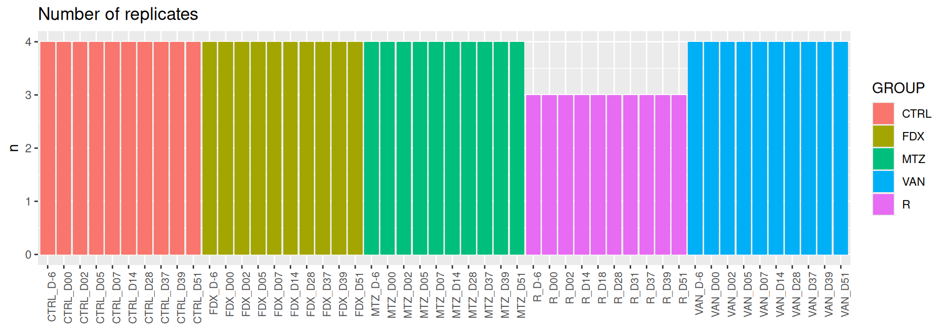
# count number of replicate by # - GROUP# - combination of GROUP and DAYsample_data(frogs) %>%as_tibble() %>% dplyr::count(GROUP)
# A tibble: 5 × 2
  GROUP     n
  <fct> <int>
1 CTRL     40
2 FDX      40
3 MTZ      40
4 VAN      40
5 R        30
Show the code
sample_data(frogs) %>%as_tibble() %>% dplyr::add_count(GROUP, DAY) %>% dplyr::select(GROUP, DAY, GROUPJ, n) %>%distinct() %>%ggplot(., aes(x = GROUPJ, y = n, fill = GROUP)) +geom_bar(stat ="identity") +labs(title="Number of replicates", y ="n") +theme(axis.title.x =element_blank(),axis.text.x =element_text(angle =90, size =8, hjust =1))
Show the code
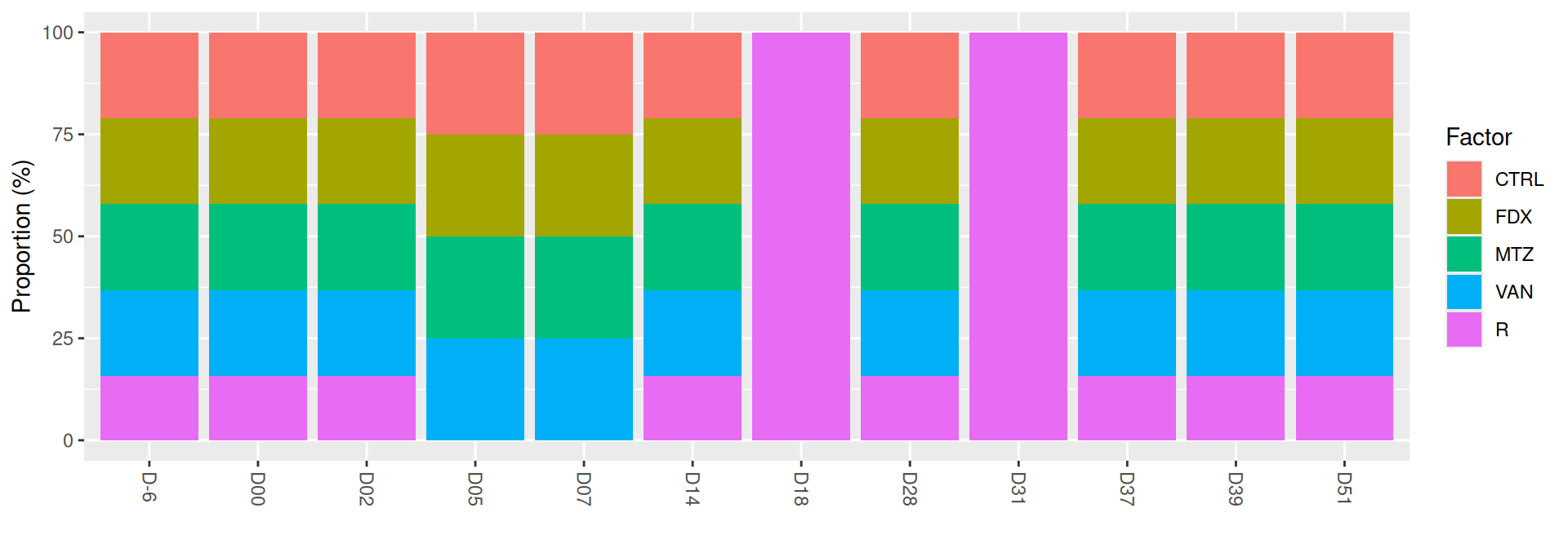
# frequencies within each DAY for the levels of GROUPmicrobiome::plot_frequencies(sample_data(frogs), "DAY", "GROUP")
Rarefaction
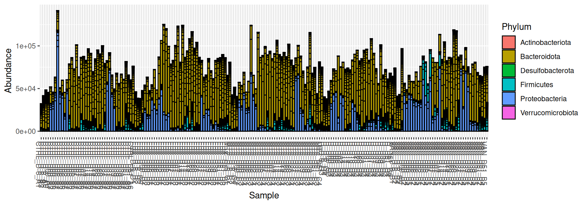
Samples from J-6 provided less abundances than the others.
Show the code
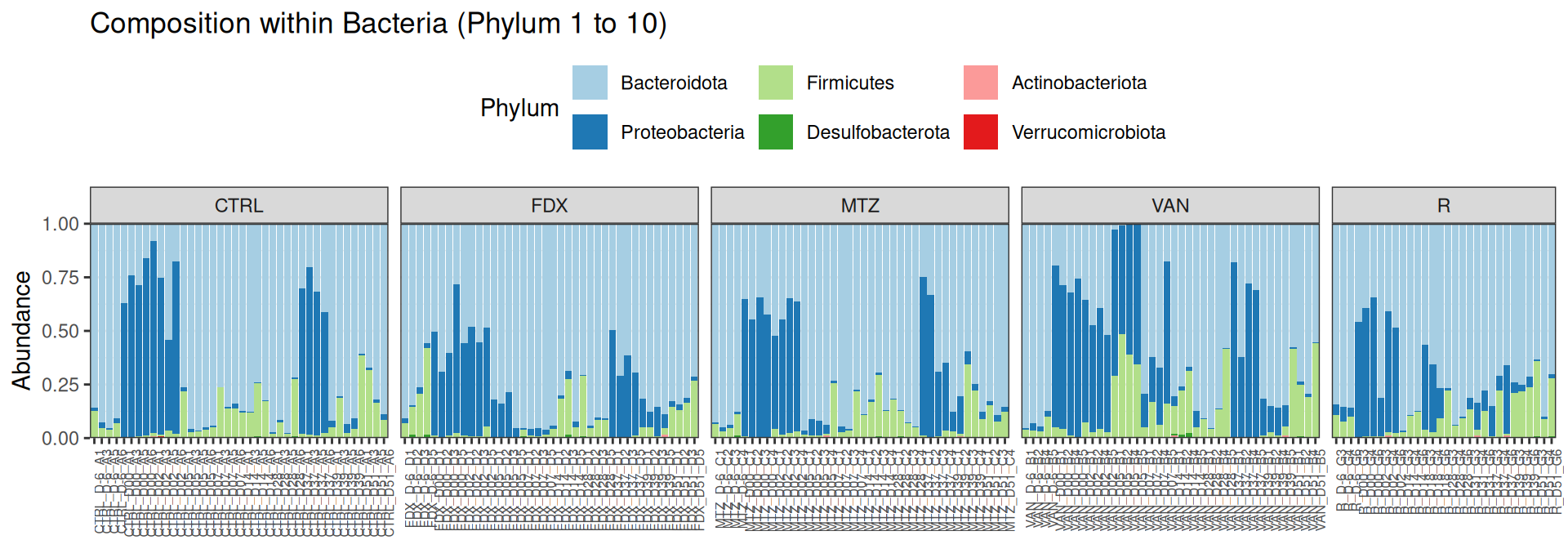
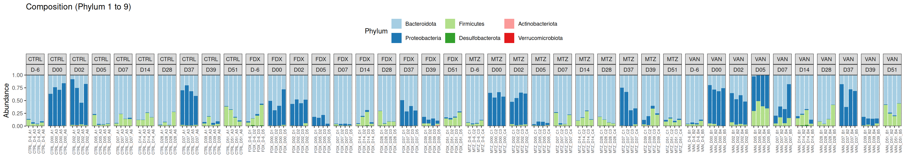
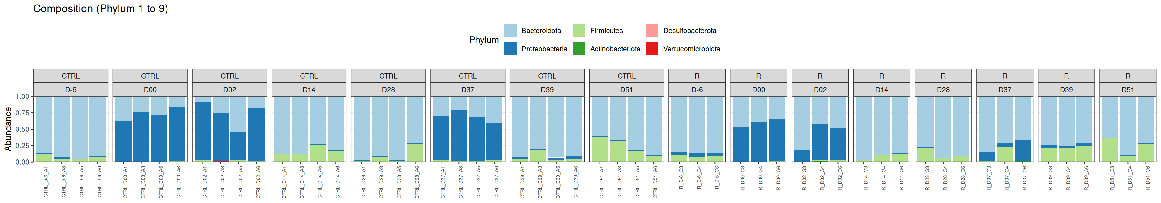
phyloseq::plot_bar(frogs, fill="Phylum")
For having the same sampling depth for all samples, we rarefy them before exploring the diversity.
The taxonomic composition is studied after rarefaction. Let’s have a look at the Phylum level composition. Fermicutes are also present up to 50% depending on the GROUP and the DAY variables. They disappear at J00, J02 J37, except J37 with R treatment.
Problematic taxa
                 taxa  Kingdom     Phylum      Class                      Order
Cluster_27 Cluster_27 Bacteria Firmicutes Clostridia Clostridia vadinBB60 group
            Family rank
Cluster_27 Unknown    9
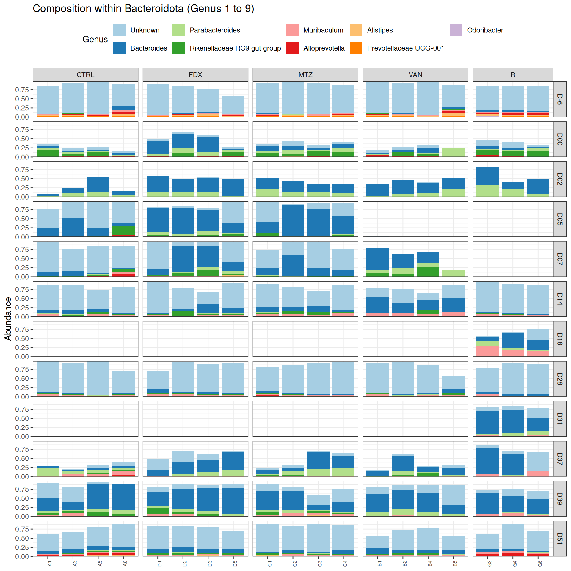
phyloseq.extended::plot_composition(frogs_rare, "Phylum", "Bacteroidota", "Genus", fill ="Genus", x ="SOURIS") +facet_grid(rows =vars(DAY), cols =vars(GROUP), scales ="free_x", space ="free_x") +scale_fill_brewer(palette ="Paired") +theme(axis.text.x =element_text(size =6, hjust =1)) +theme(legend.position="top")
Problematic taxa
taxa Kingdom Phylum Class Order
Cluster_3 Cluster_3 Bacteria Bacteroidota Bacteroidia Bacteroidales
Family Genus rank
Cluster_3 Muribaculaceae Unknown 1
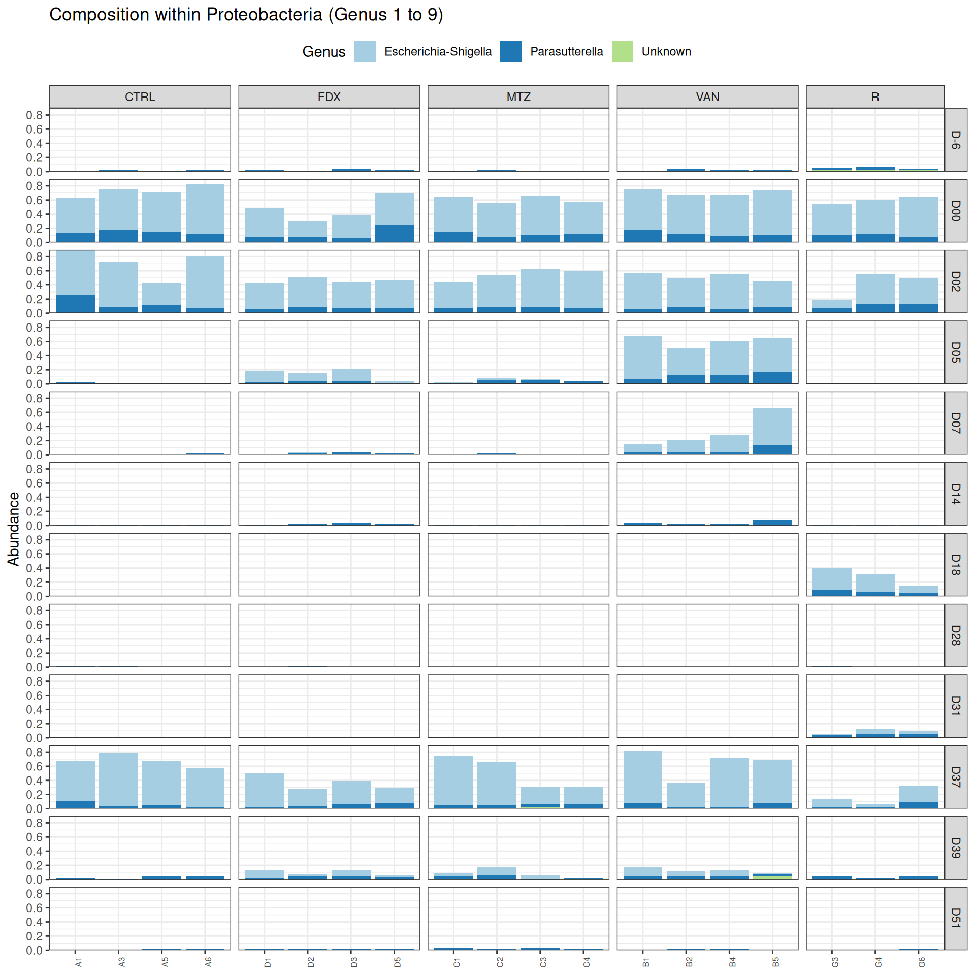
Show the code
phyloseq.extended::plot_composition(frogs_rare, "Phylum", "Proteobacteria", "Genus", fill ="Genus", x ="SOURIS") +facet_grid(rows =vars(DAY), cols =vars(GROUP), scales ="free_x", space ="free_x") +scale_fill_brewer(palette ="Paired") +theme(axis.text.x =element_text(size =6, hjust =1)) +theme(legend.position="top")
Problematic taxa
taxa Kingdom Phylum Class
Cluster_51 Cluster_51 Bacteria Proteobacteria Alphaproteobacteria
Order Family Genus rank
Cluster_51 Rhodospirillales Unknown Unknown 3
Show the code
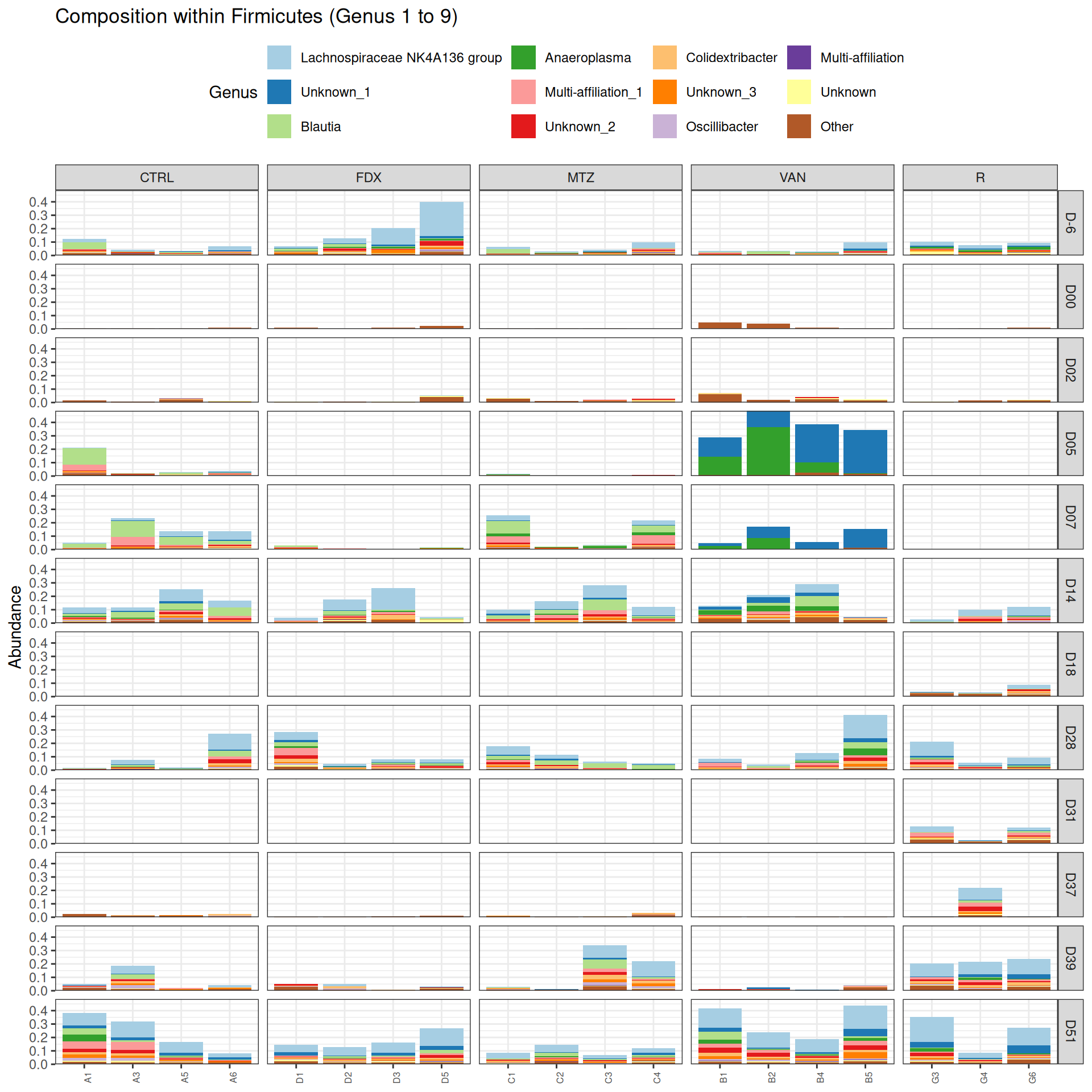
phyloseq.extended::plot_composition(frogs_rare, "Phylum", "Firmicutes", "Genus", fill ="Genus", x ="SOURIS") +facet_grid(rows =vars(DAY), cols =vars(GROUP), scales ="free_x", space ="free_x") +scale_fill_brewer(palette ="Paired") +theme(axis.text.x =element_text(size =6, hjust =1)) +theme(legend.position="top")
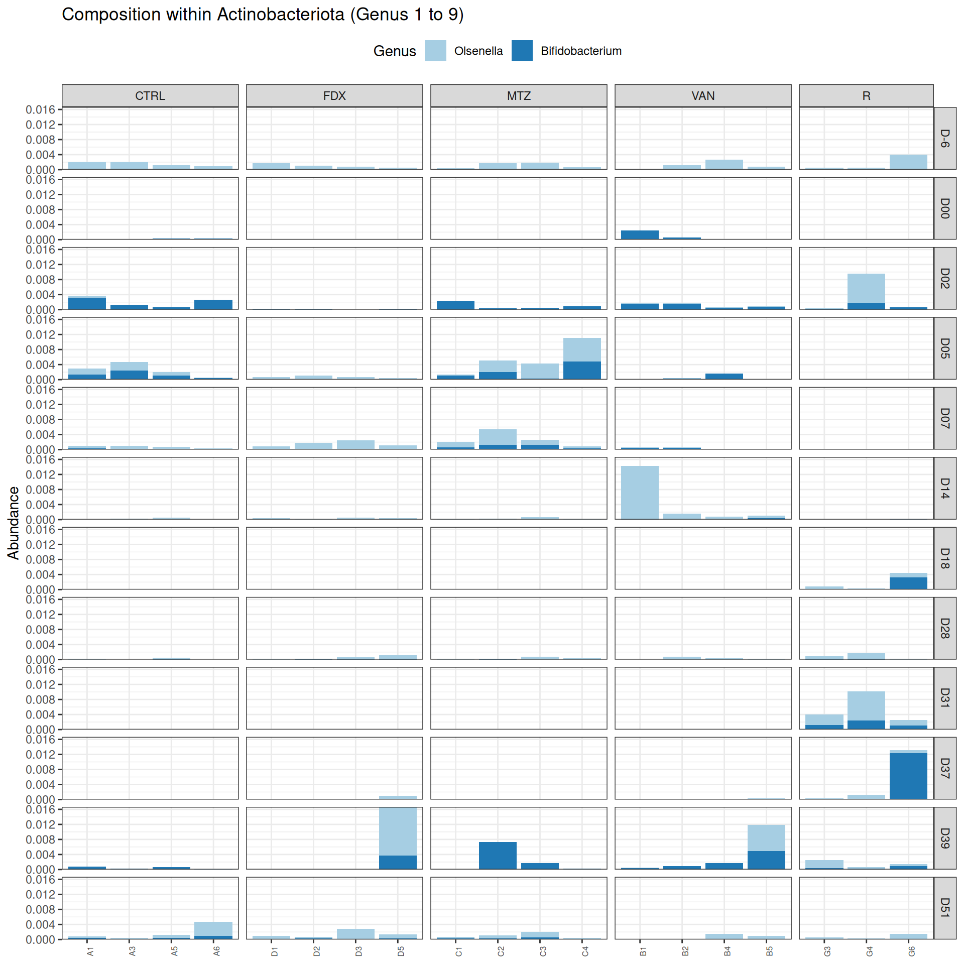
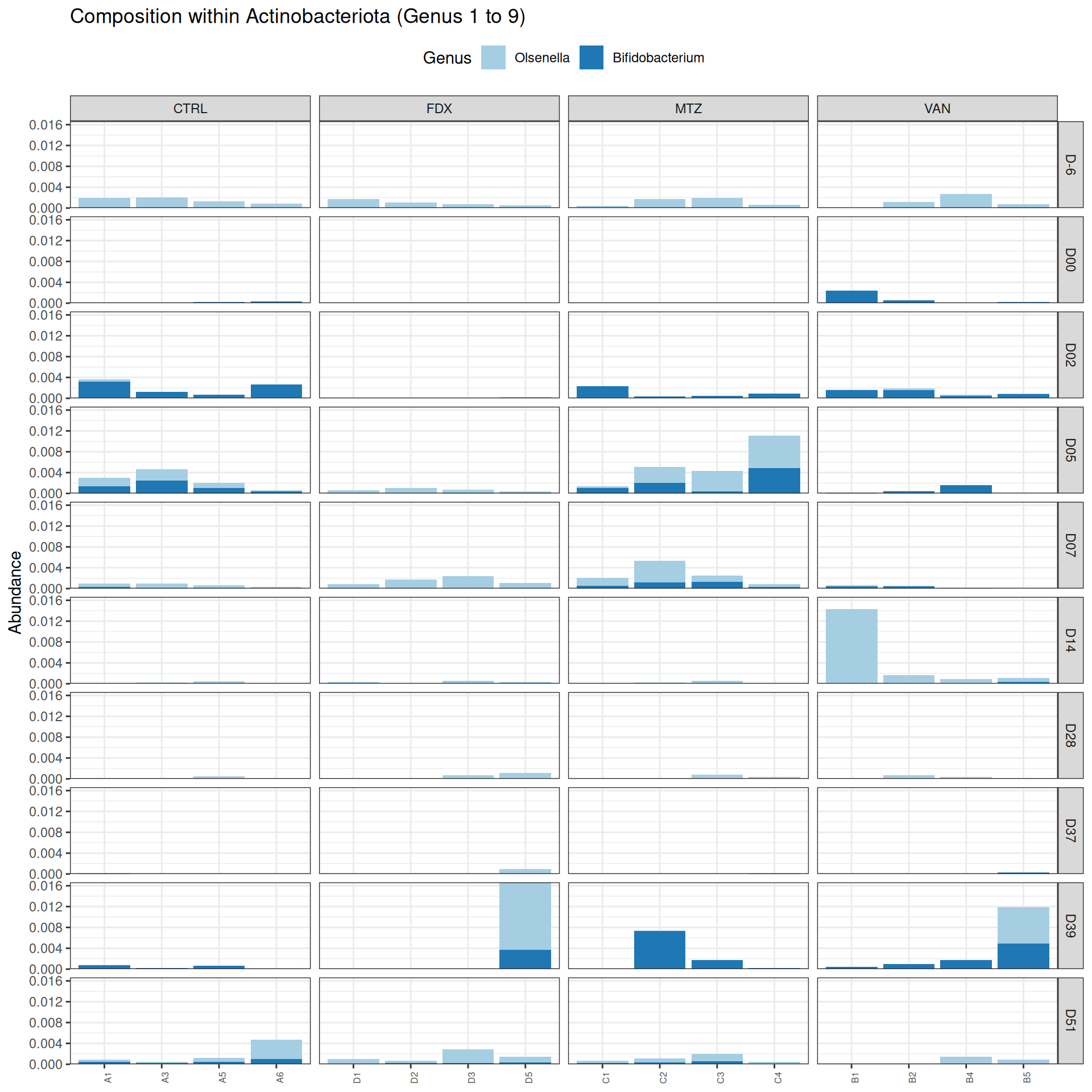
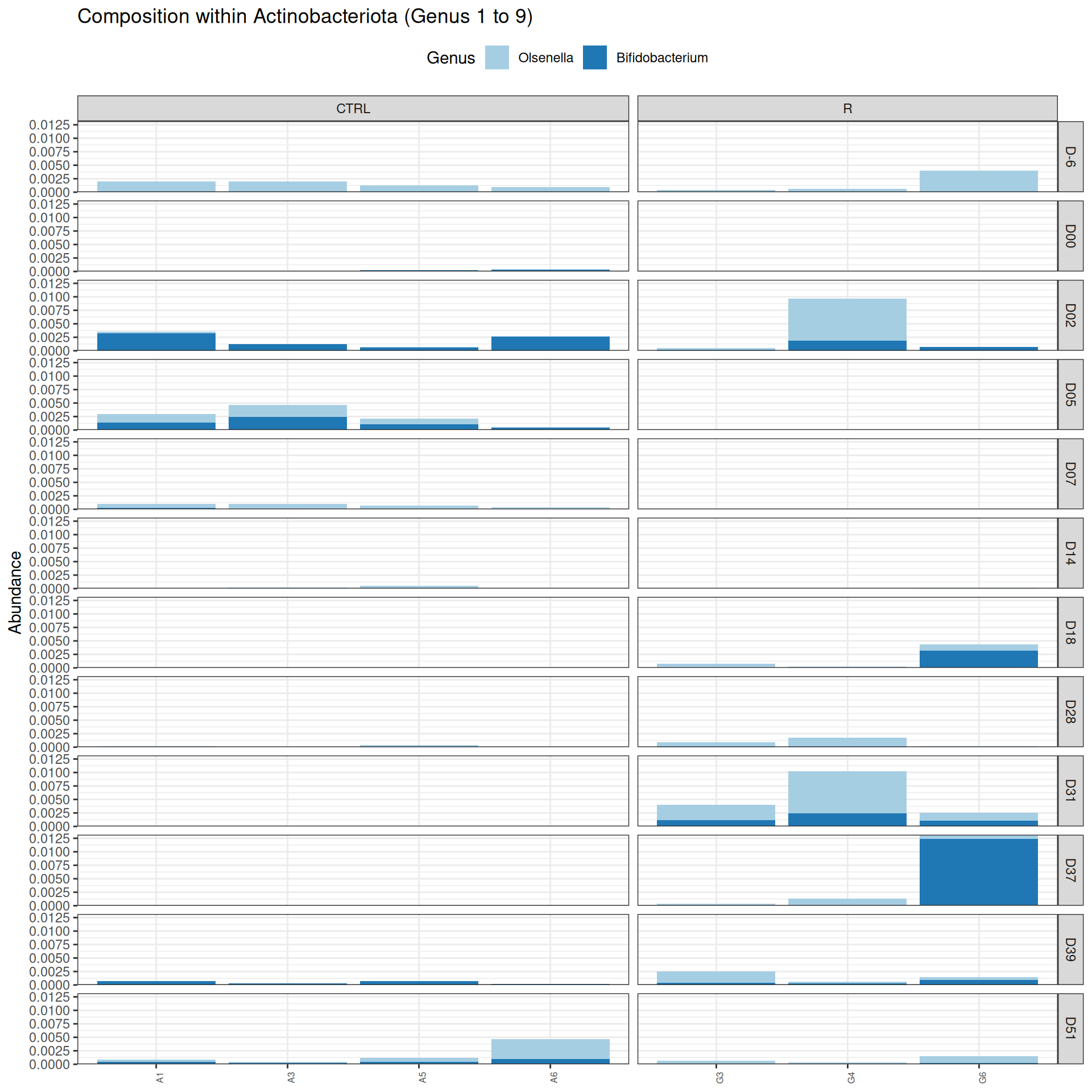
phyloseq.extended::plot_composition(frogs_rare, "Phylum", "Actinobacteriota", "Genus", fill ="Genus", x ="SOURIS") +facet_grid(rows =vars(DAY), cols =vars(GROUP), scales ="free_x", space ="free_x") +scale_fill_brewer(palette ="Paired") +theme(axis.text.x =element_text(size =6, hjust =1)) +theme(legend.position="top")
Show the code
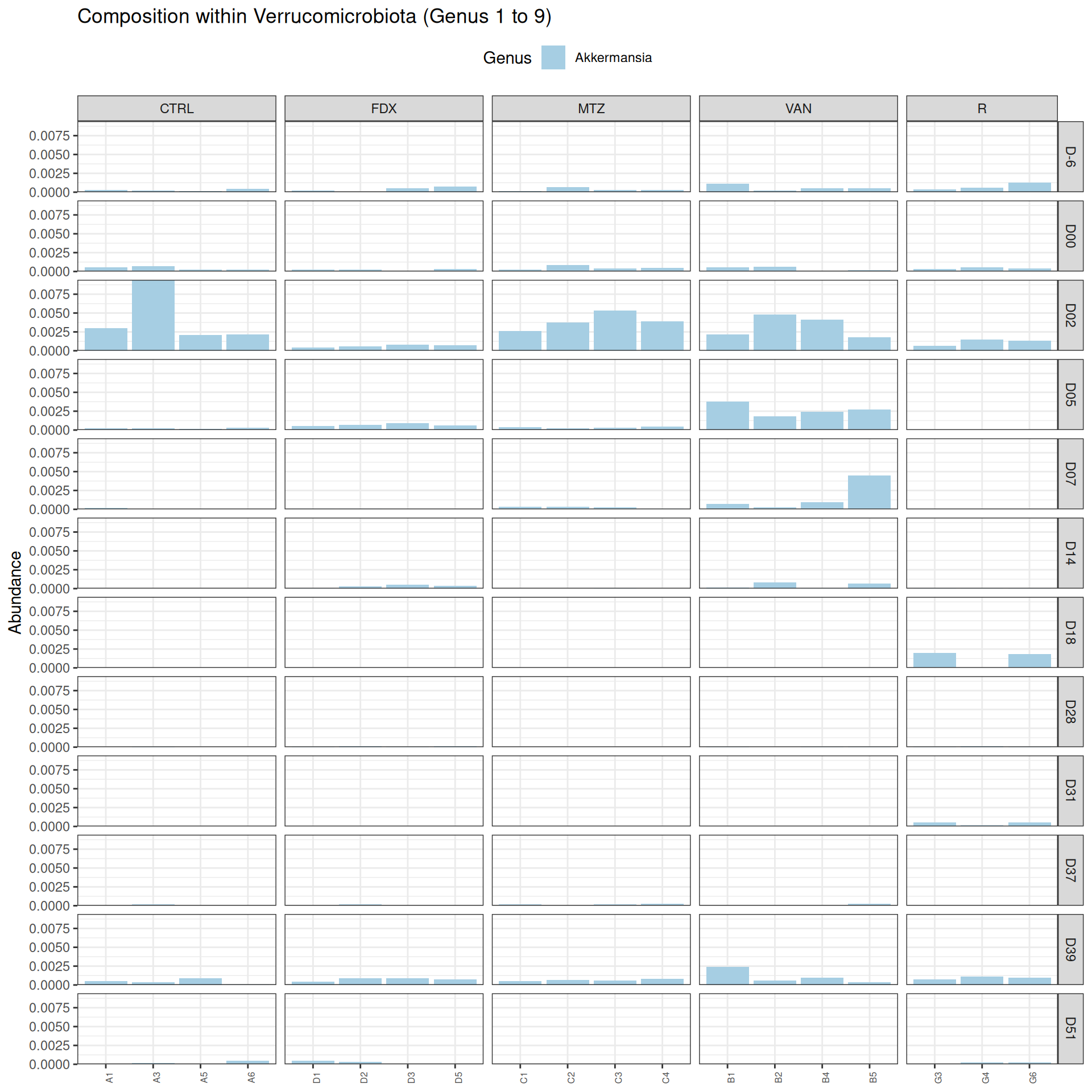
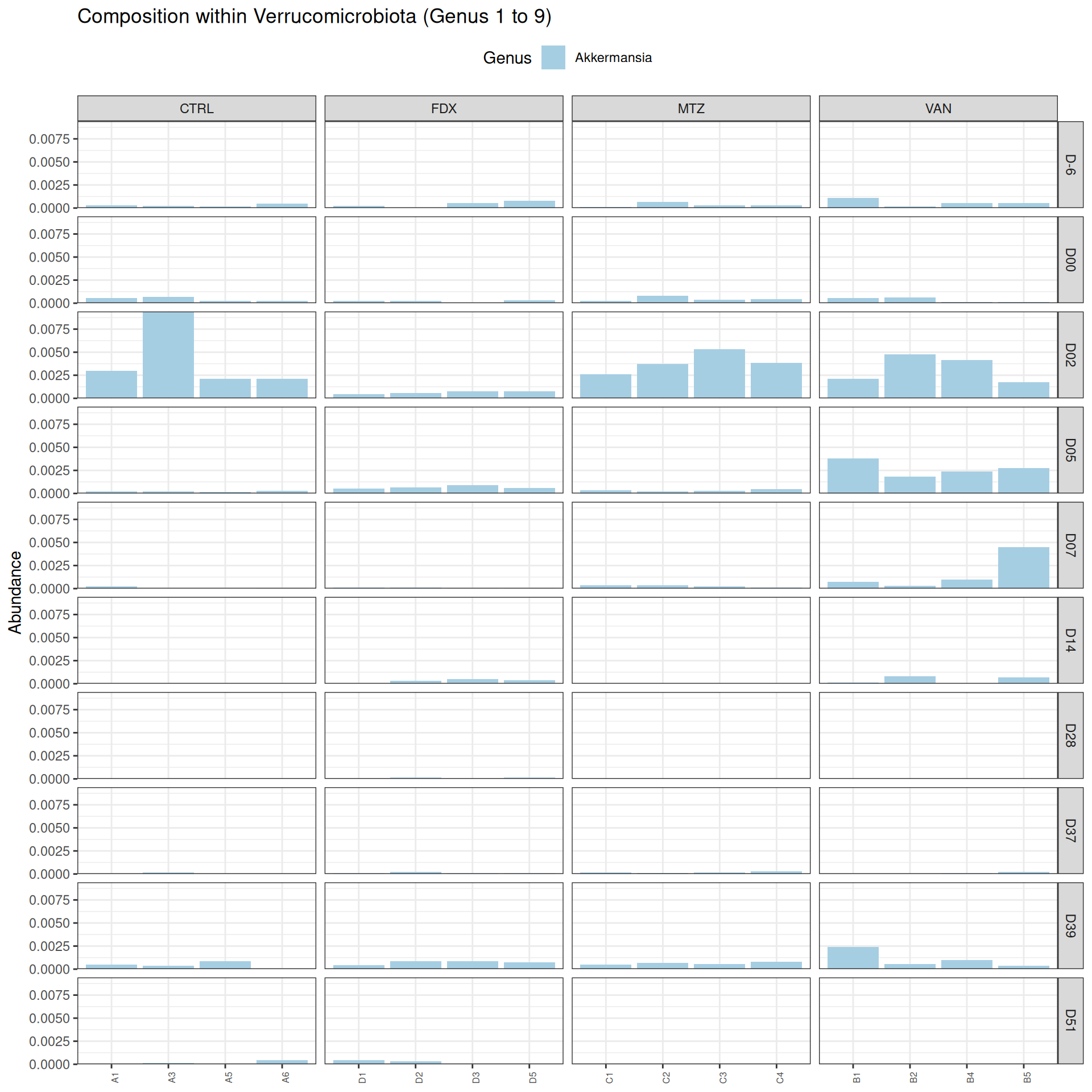
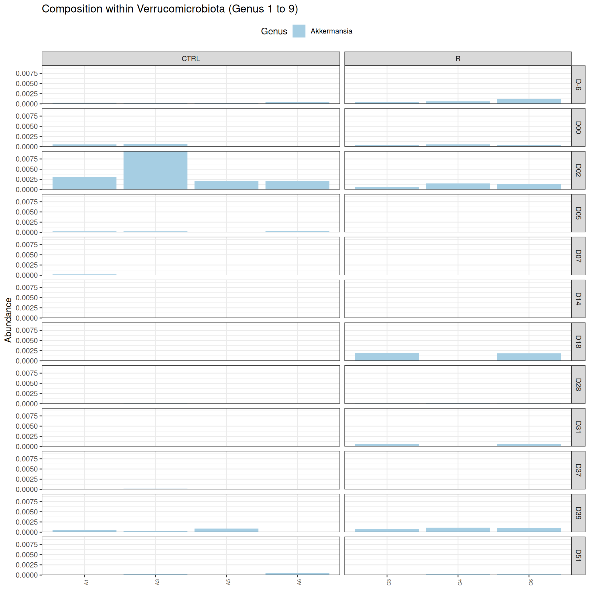
phyloseq.extended::plot_composition(frogs_rare, "Phylum", "Verrucomicrobiota", "Genus", fill ="Genus", x ="SOURIS") +facet_grid(rows =vars(DAY), cols =vars(GROUP), scales ="free_x", space ="free_x") +scale_fill_brewer(palette ="Paired") +theme(axis.text.x =element_text(size =6, hjust =1)) +theme(legend.position="top")
Important
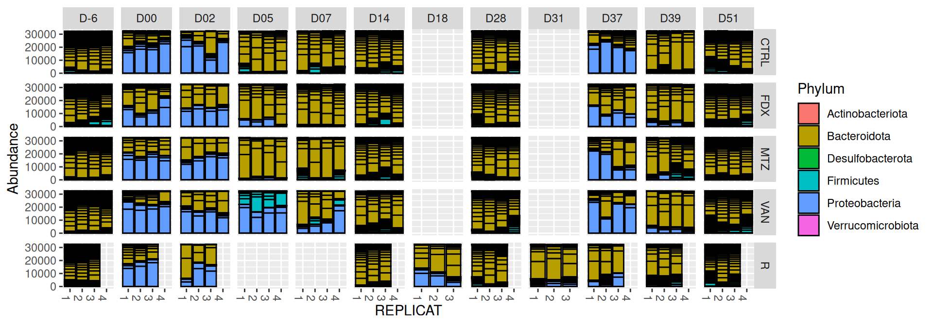
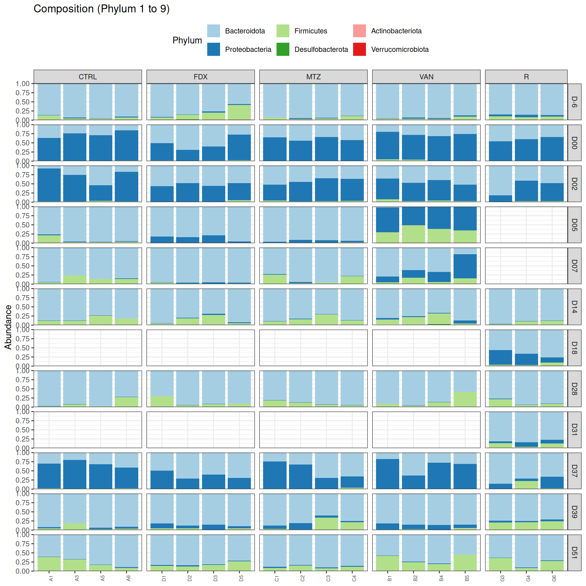
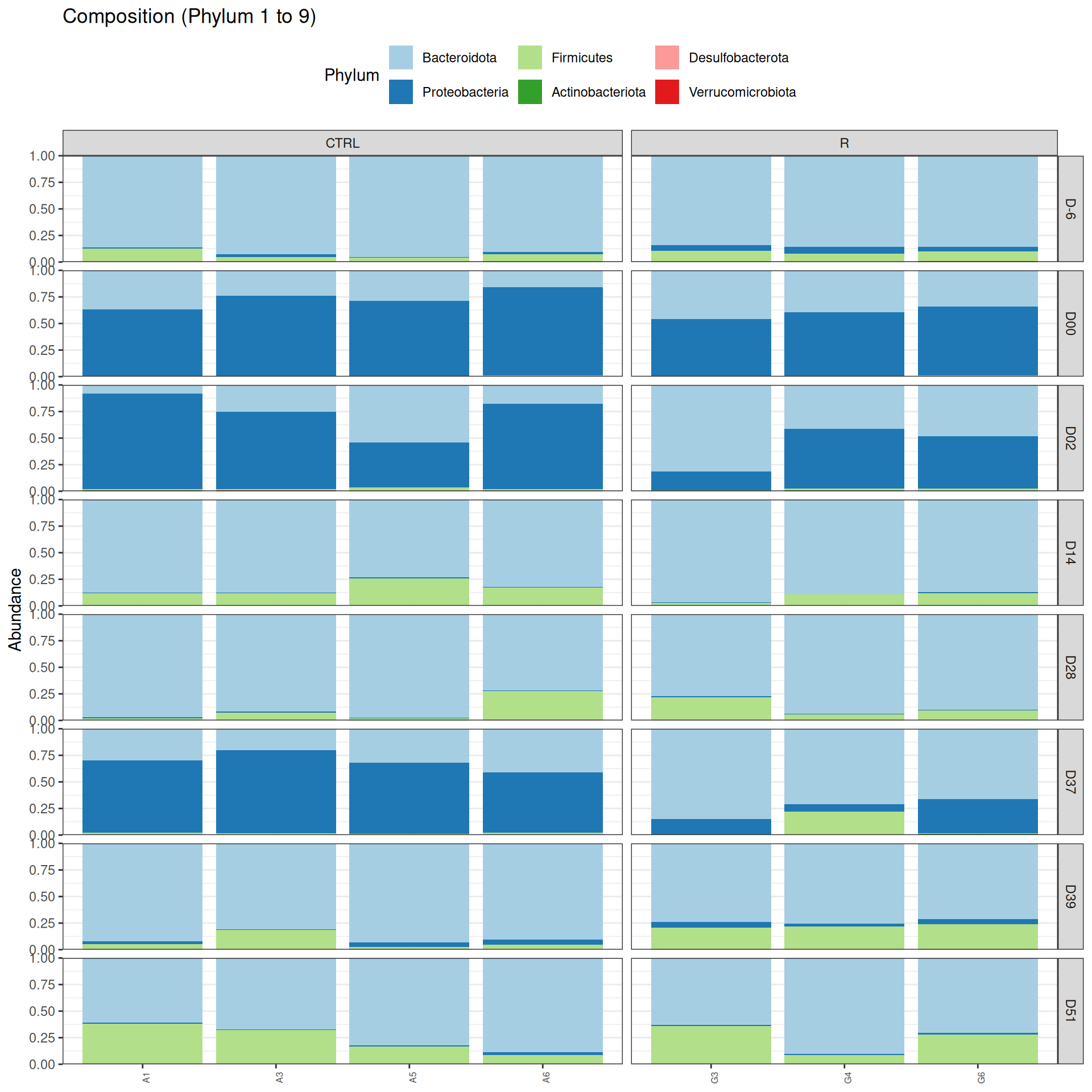
We observed that the taxonomic composition is mainly determined by DAY rather than GROUP. Protebacteria are dominant in J00, J02, J18 (GROUP R) and J37. Firmicutes are present at J-6 (a little), J05 (CTRL and VAN), J07 (CTRL, VAN, MTZ), J14, J28, J39, J51. At the genus level, similar taxonomic patterns were found in J00 with J37 and in J-6 with J51.
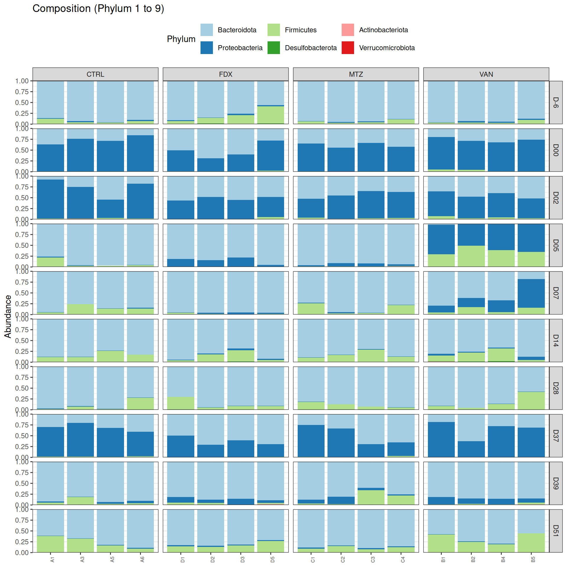
phyloseq.extended::plot_composition(physeq =subset_samples(frogs_rare, GROUP !="R"), NULL, NULL, "Phylum") +facet_grid(~ GROUP + DAY, scales ="free_x", space ="free_x") +scale_fill_brewer(palette ="Paired") +theme(axis.text.x =element_text(size =6, hjust =1)) +theme(legend.position="top")
Show the code
phyloseq.extended::plot_composition(physeq =subset_samples(frogs_rare, GROUP !="R"), NULL, NULL, "Phylum", x ="SOURIS") +facet_grid(rows =vars(DAY), cols =vars(GROUP), scales ="free_x", space ="free_x") +scale_fill_brewer(palette ="Paired") +theme(axis.text.x =element_text(size =6, hjust =1)) +theme(legend.position="top")
Show the code
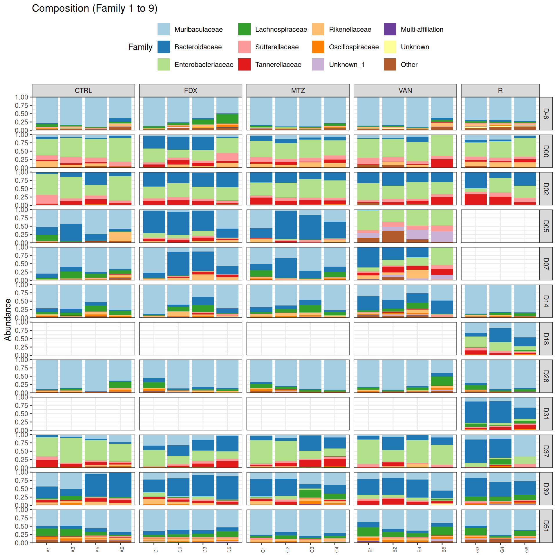
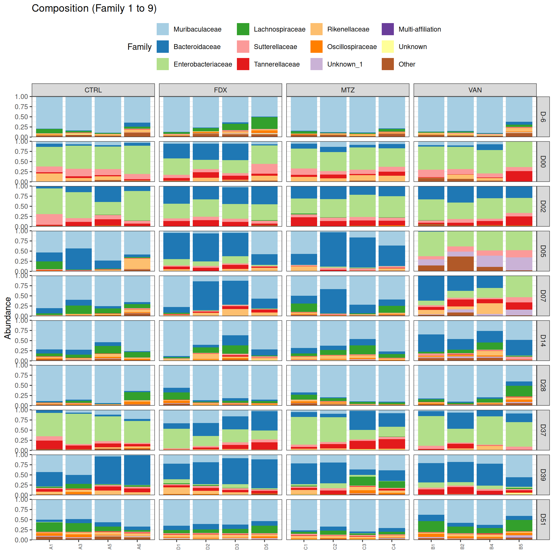
phyloseq.extended::plot_composition(physeq =subset_samples(frogs_rare, GROUP !="R"), NULL, NULL, "Family", x ="SOURIS") +facet_grid(rows =vars(DAY), cols =vars(GROUP), scales ="free_x", space ="free_x") +scale_fill_brewer(palette ="Paired") +theme(axis.text.x =element_text(size =6, hjust =1)) +theme(legend.position="top")
Problematic taxa
taxa Kingdom Phylum Class Order
Cluster_27 Cluster_27 Bacteria Firmicutes Clostridia Clostridia vadinBB60 group
Family rank
Cluster_27 Unknown 9
Show the code
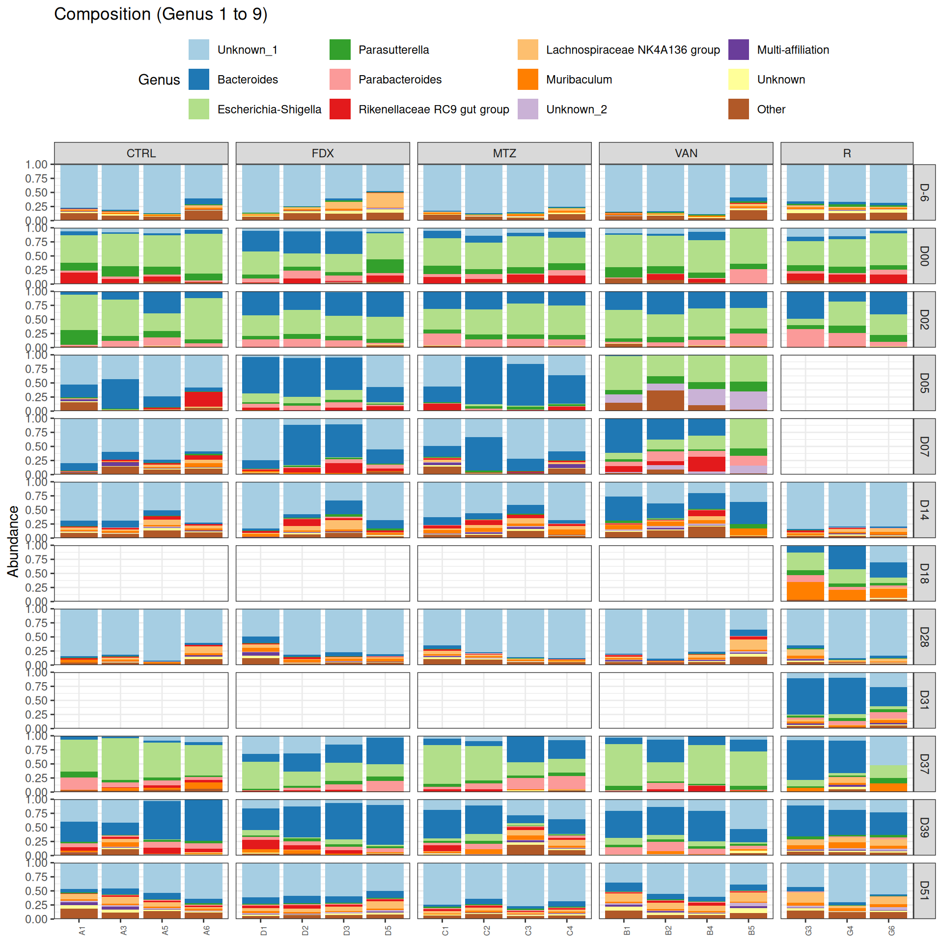
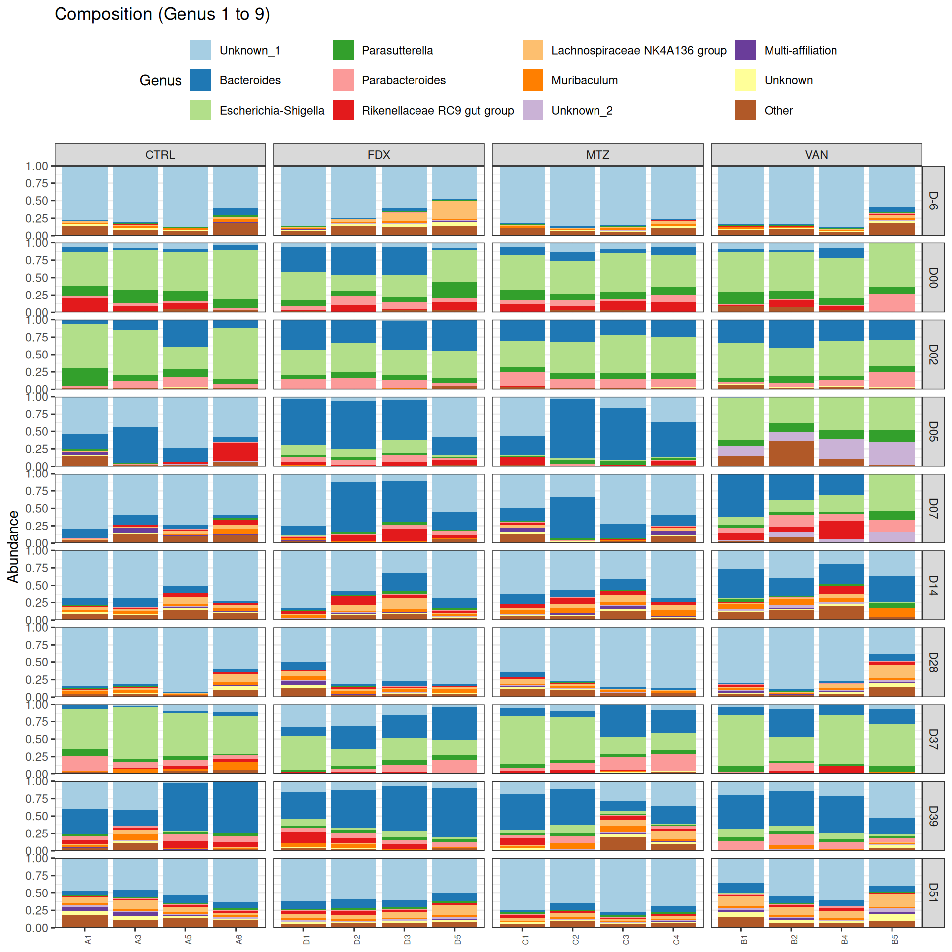
phyloseq.extended::plot_composition(physeq =subset_samples(frogs_rare, GROUP !="R"), NULL, NULL, "Genus", x ="SOURIS") +facet_grid(rows =vars(DAY), cols =vars(GROUP), scales ="free_x", space ="free_x") +scale_fill_brewer(palette ="Paired") +theme(axis.text.x =element_text(size =6, hjust =1)) +theme(legend.position="top")
Problematic taxa
                 taxa  Kingdom       Phylum       Class
Cluster_3   Cluster_3 Bacteria Bacteroidota Bacteroidia
Cluster_27 Cluster_27 Bacteria   Firmicutes  Clostridia
                                Order         Family   Genus rank
Cluster_3               Bacteroidales Muribaculaceae Unknown    1
Cluster_27 Clostridia vadinBB60 group        Unknown Unknown    9
To explore presence of bacteria at genus levels within phylum:
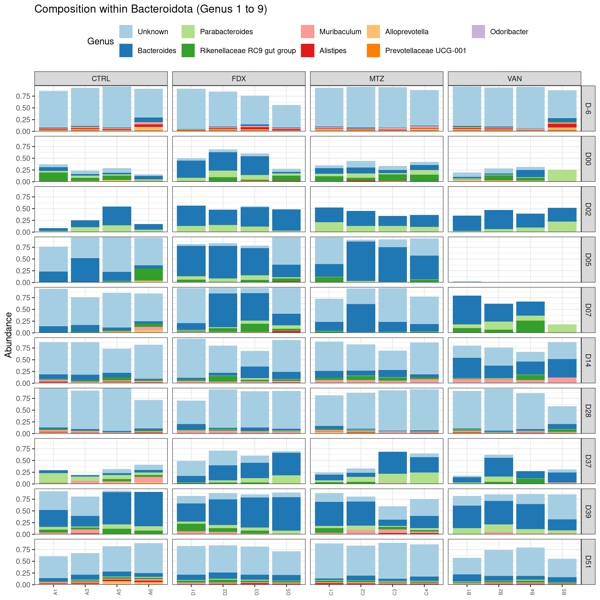
phyloseq.extended::plot_composition(physeq =subset_samples(frogs_rare, GROUP !="R"), "Phylum", "Bacteroidota", "Genus", fill ="Genus", x ="SOURIS") +facet_grid(rows =vars(DAY), cols =vars(GROUP), scales ="free_x", space ="free_x") +scale_fill_brewer(palette ="Paired") +theme(axis.text.x =element_text(size =6, hjust =1)) +theme(legend.position="top")
Problematic taxa
               taxa  Kingdom       Phylum       Class         Order
Cluster_3 Cluster_3 Bacteria Bacteroidota Bacteroidia Bacteroidales
                  Family   Genus rank
Cluster_3 Muribaculaceae Unknown    1
Show the code
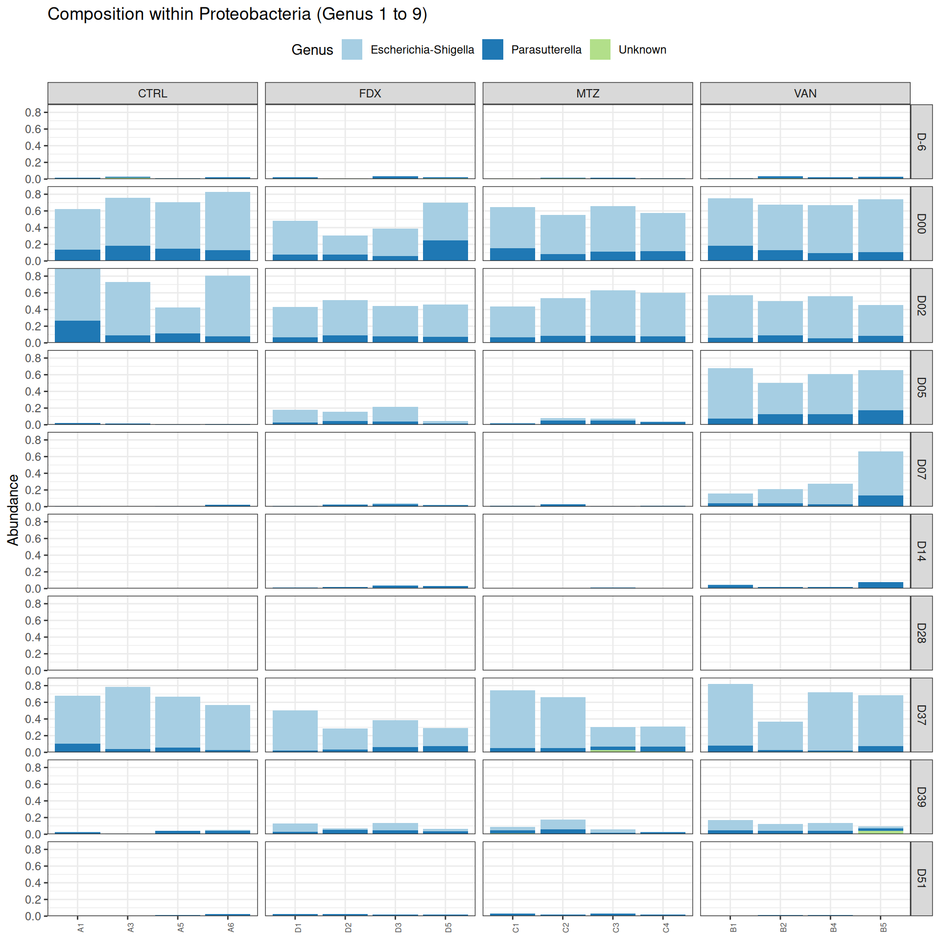
phyloseq.extended::plot_composition(physeq =subset_samples(frogs_rare, GROUP !="R"), "Phylum", "Proteobacteria", "Genus", fill ="Genus", x ="SOURIS") +facet_grid(rows =vars(DAY), cols =vars(GROUP), scales ="free_x", space ="free_x") +scale_fill_brewer(palette ="Paired") +theme(axis.text.x =element_text(size =6, hjust =1)) +theme(legend.position="top")
Problematic taxa
                 taxa  Kingdom         Phylum               Class
Cluster_51 Cluster_51 Bacteria Proteobacteria Alphaproteobacteria
                      Order  Family   Genus rank
Cluster_51 Rhodospirillales Unknown Unknown    3
Show the code
phyloseq.extended::plot_composition(physeq =subset_samples(frogs_rare, GROUP !="R"), "Phylum", "Firmicutes", "Genus", fill ="Genus", x ="SOURIS") +facet_grid(rows =vars(DAY), cols =vars(GROUP), scales ="free_x", space ="free_x") +scale_fill_brewer(palette ="Paired") +theme(axis.text.x =element_text(size =6, hjust =1)) +theme(legend.position="top")
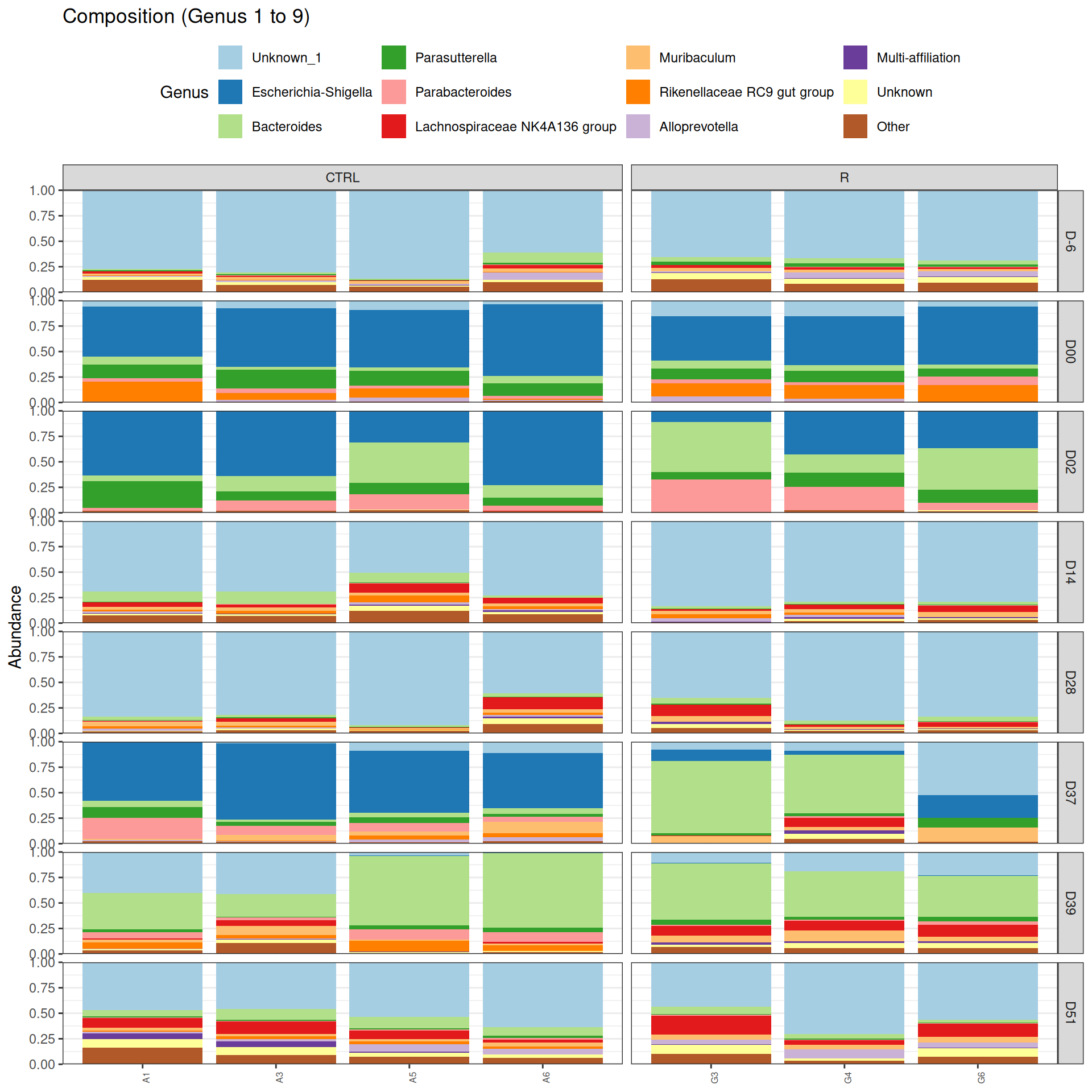
phyloseq.extended::plot_composition(physeq =subset_samples(frogs_rare, DAY %in%c("D-6", "D00", "D02", "D14", "D28", "D37", "D39", "D51") & GROUP %in%c("R", "CTRL")), NULL, NULL, "Phylum") +facet_grid(~ GROUP + DAY, scales ="free_x", space ="free_x") +scale_fill_brewer(palette ="Paired") +theme(axis.text.x =element_text(size =6, hjust =1)) +theme(legend.position="top")
Show the code
phyloseq.extended::plot_composition(physeq =subset_samples(frogs_rare, DAY %in%c("D-6", "D00", "D02", "D14", "D28", "D37", "D39", "D51") & GROUP %in%c("R", "CTRL")), NULL, NULL, "Phylum", x ="SOURIS") +facet_grid(rows =vars(DAY), cols =vars(GROUP), scales ="free_x", space ="free_x") +scale_fill_brewer(palette ="Paired") +theme(axis.text.x =element_text(size =6, hjust =1)) +theme(legend.position="top")
Show the code
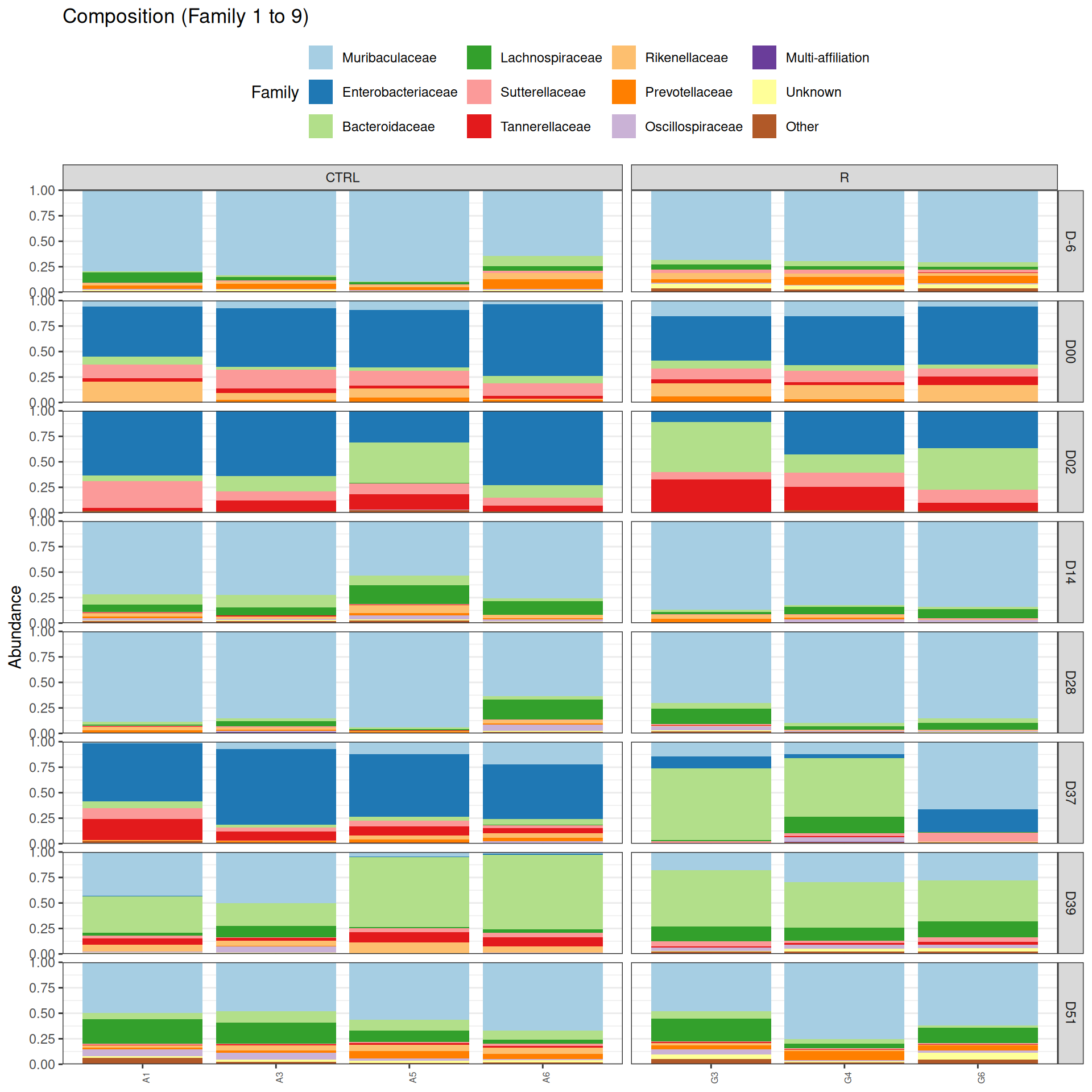
phyloseq.extended::plot_composition(physeq =subset_samples(frogs_rare, DAY %in%c("D-6", "D00", "D02", "D14", "D28", "D37", "D39", "D51") & GROUP %in%c("R", "CTRL")), NULL, NULL, "Family", x ="SOURIS") +facet_grid(rows =vars(DAY), cols =vars(GROUP), scales ="free_x", space ="free_x") +scale_fill_brewer(palette ="Paired") +theme(axis.text.x =element_text(size =6, hjust =1)) +theme(legend.position="top")
Show the code
phyloseq.extended::plot_composition(physeq =subset_samples(frogs_rare, DAY %in%c("D-6", "D00", "D02", "D14", "D28", "D37", "D39", "D51") & GROUP %in%c("R", "CTRL")), NULL, NULL, "Genus", x ="SOURIS") +facet_grid(rows =vars(DAY), cols =vars(GROUP), scales ="free_x", space ="free_x") +scale_fill_brewer(palette ="Paired") +theme(axis.text.x =element_text(size =6, hjust =1)) +theme(legend.position="top")
Problematic taxa
               taxa  Kingdom       Phylum       Class         Order
Cluster_3 Cluster_3 Bacteria Bacteroidota Bacteroidia Bacteroidales
                  Family   Genus rank
Cluster_3 Muribaculaceae Unknown    1
To explore presence of bacteria at genus levels within phylum:
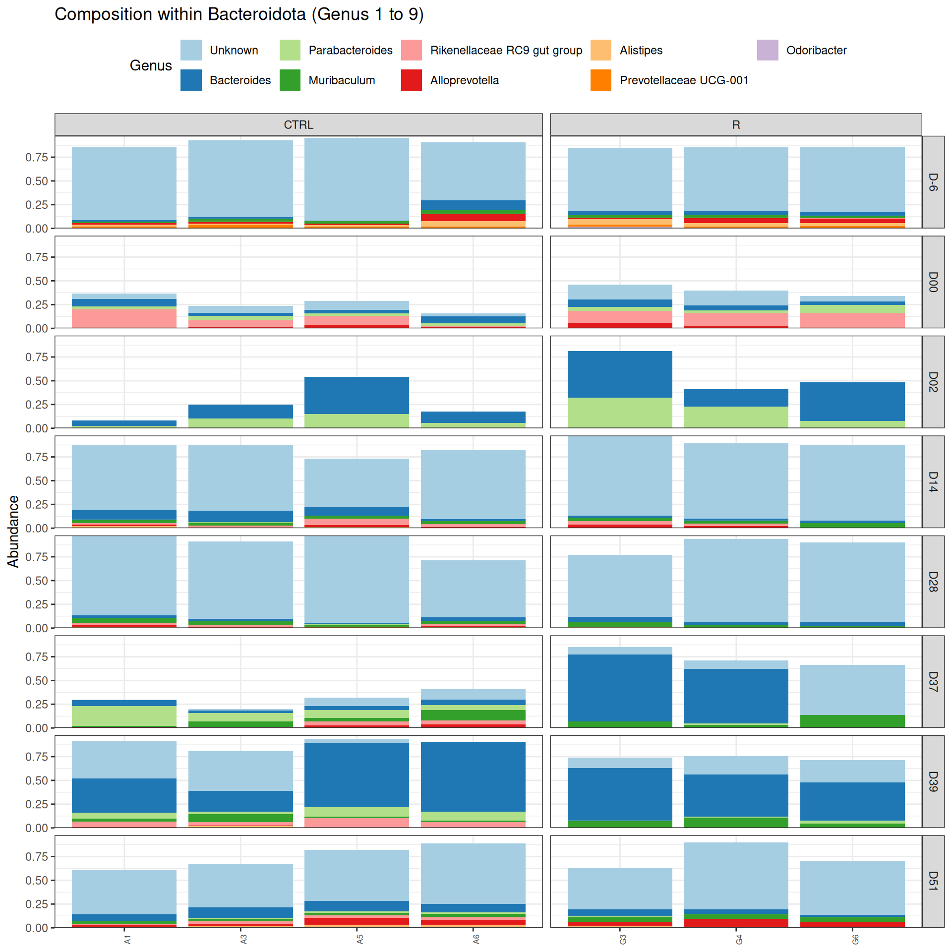
phyloseq.extended::plot_composition(physeq =subset_samples(frogs_rare, DAY %in%c("D-6", "D00", "D02", "D14", "D28", "D37", "D39", "D51") & GROUP %in%c("R", "CTRL")), "Phylum", "Bacteroidota", "Genus", fill ="Genus", x ="SOURIS") +facet_grid(rows =vars(DAY), cols =vars(GROUP), scales ="free_x", space ="free_x") +scale_fill_brewer(palette ="Paired") +theme(axis.text.x =element_text(size =6, hjust =1)) +theme(legend.position="top")
Problematic taxa
taxa Kingdom Phylum Class Order
Cluster_3 Cluster_3 Bacteria Bacteroidota Bacteroidia Bacteroidales
Family Genus rank
Cluster_3 Muribaculaceae Unknown 1
Show the code
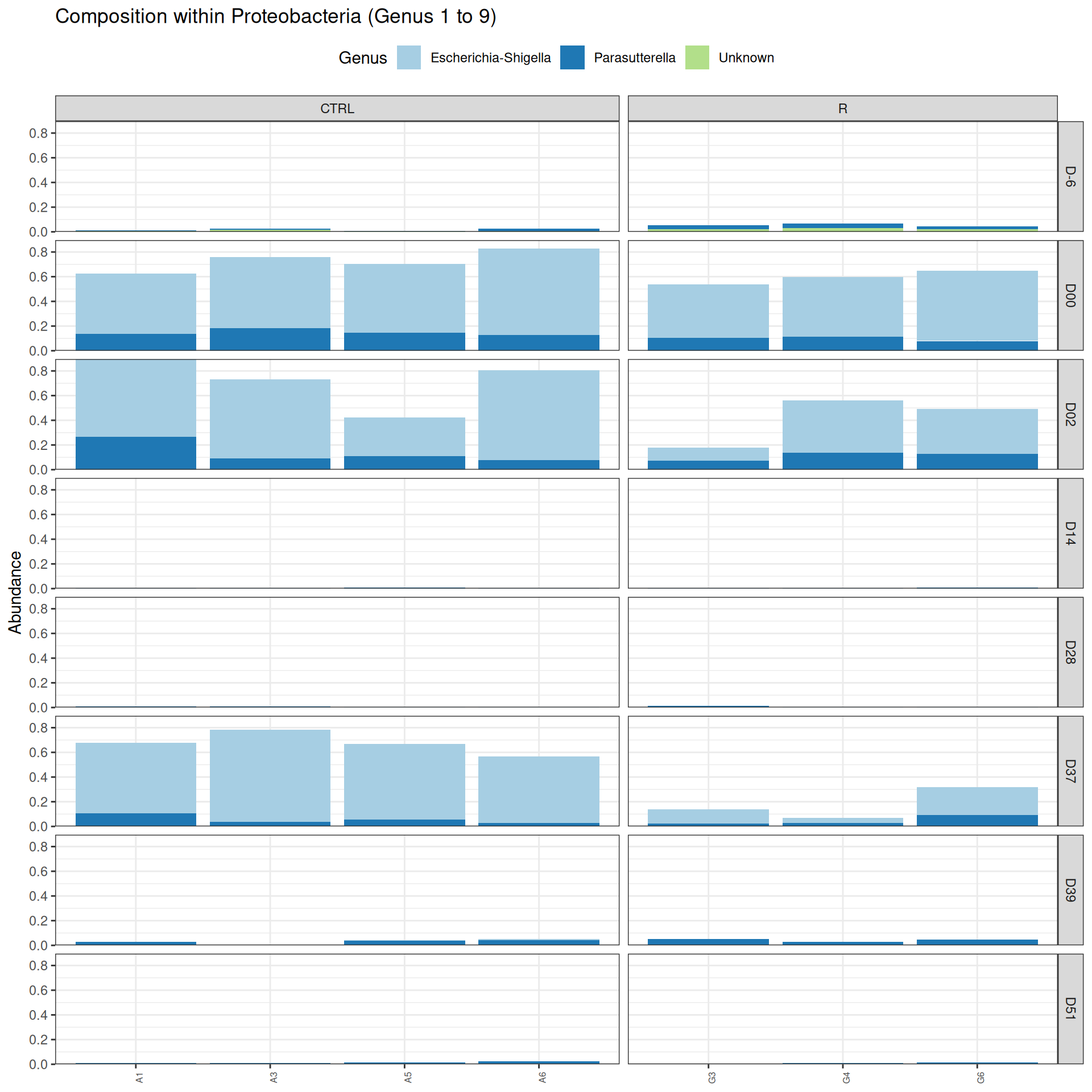
phyloseq.extended::plot_composition(physeq =subset_samples(frogs_rare, DAY %in%c("D-6", "D00", "D02", "D14", "D28", "D37", "D39", "D51") & GROUP %in%c("R", "CTRL")), "Phylum", "Proteobacteria", "Genus", fill ="Genus", x ="SOURIS") +facet_grid(rows =vars(DAY), cols =vars(GROUP), scales ="free_x", space ="free_x") +scale_fill_brewer(palette ="Paired") +theme(axis.text.x =element_text(size =6, hjust =1)) +theme(legend.position="top")
Problematic taxa
                 taxa  Kingdom         Phylum               Class
Cluster_51 Cluster_51 Bacteria Proteobacteria Alphaproteobacteria
                      Order  Family   Genus rank
Cluster_51 Rhodospirillales Unknown Unknown    3
Show the code
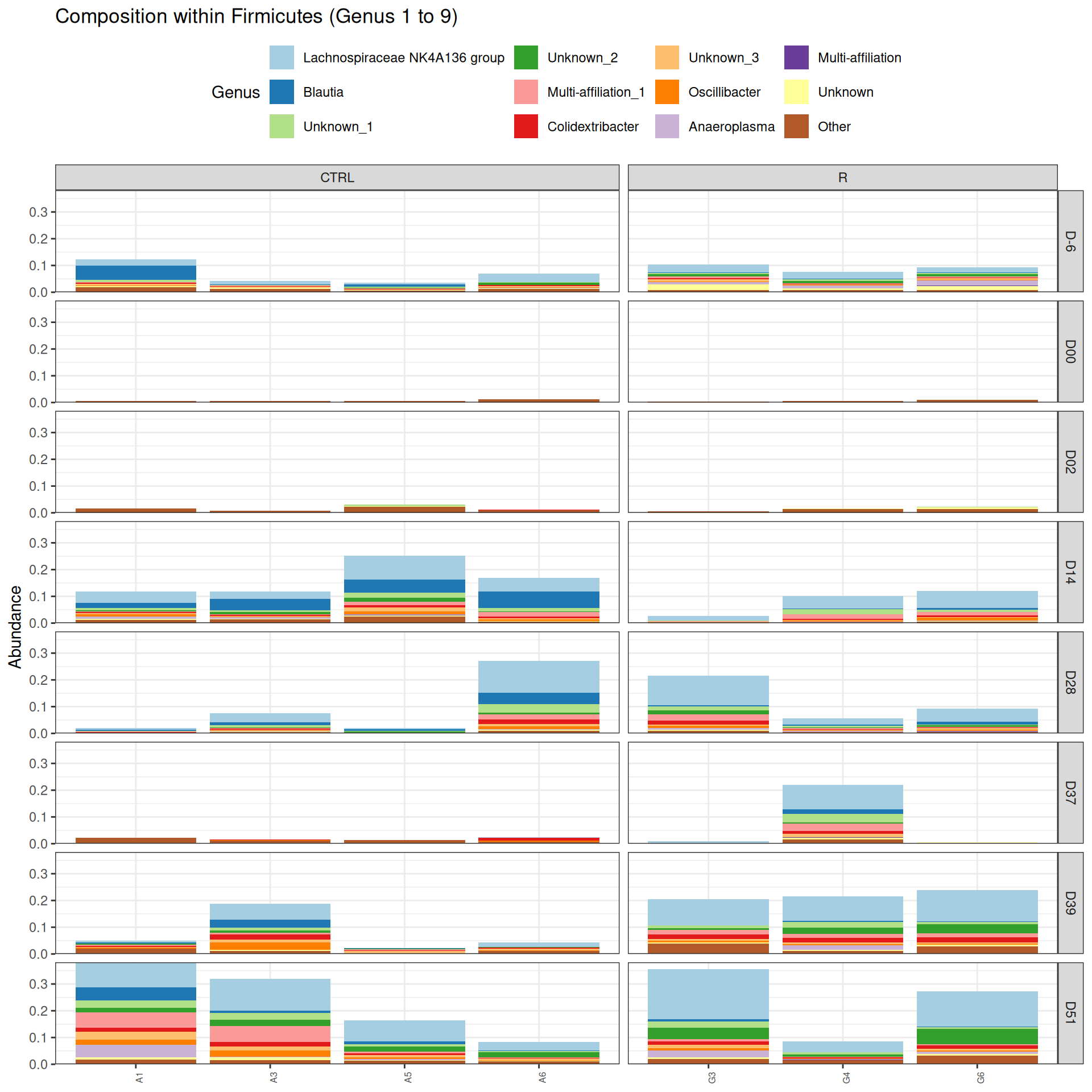
phyloseq.extended::plot_composition(physeq =subset_samples(frogs_rare, DAY %in%c("D-6", "D00", "D02", "D14", "D28", "D37", "D39", "D51") & GROUP %in%c("R", "CTRL")), "Phylum", "Firmicutes", "Genus", fill ="Genus", x ="SOURIS") +facet_grid(rows =vars(DAY), cols =vars(GROUP), scales ="free_x", space ="free_x") +scale_fill_brewer(palette ="Paired") +theme(axis.text.x =element_text(size =6, hjust =1)) +theme(legend.position="top")
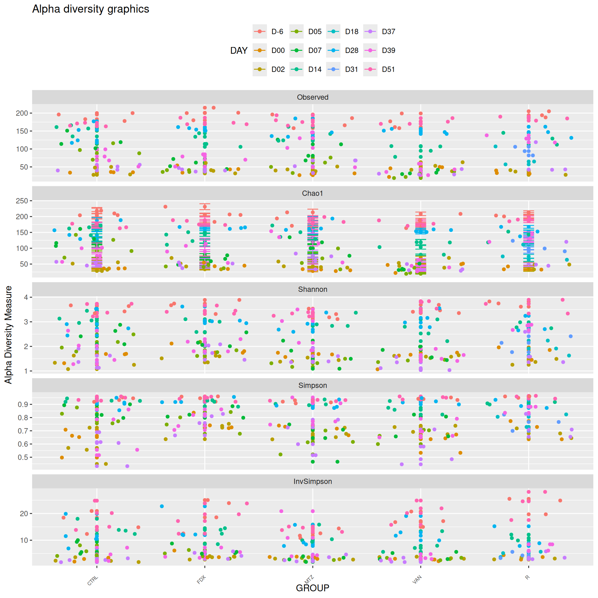
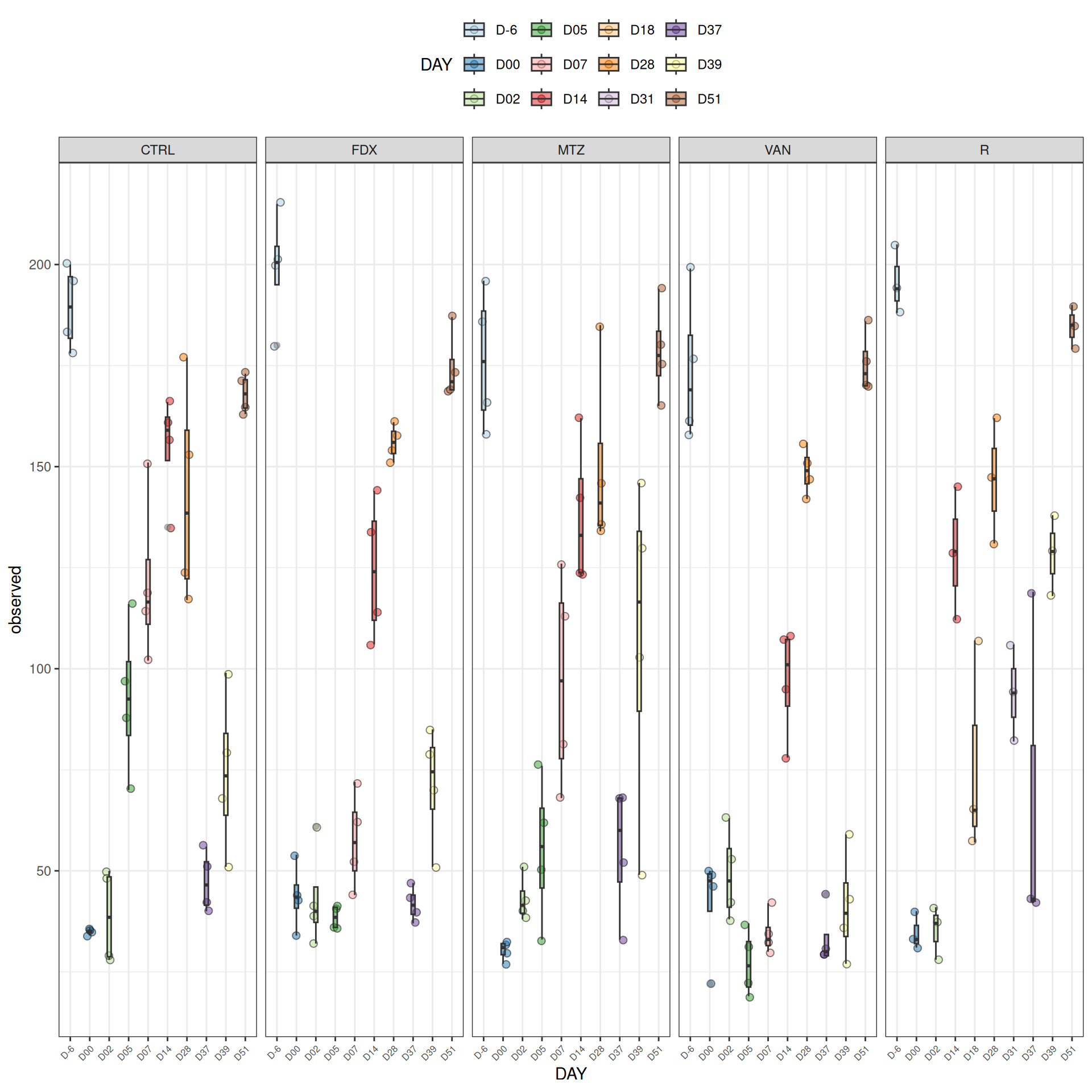
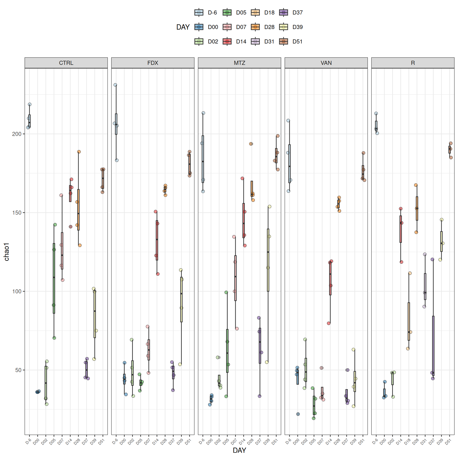
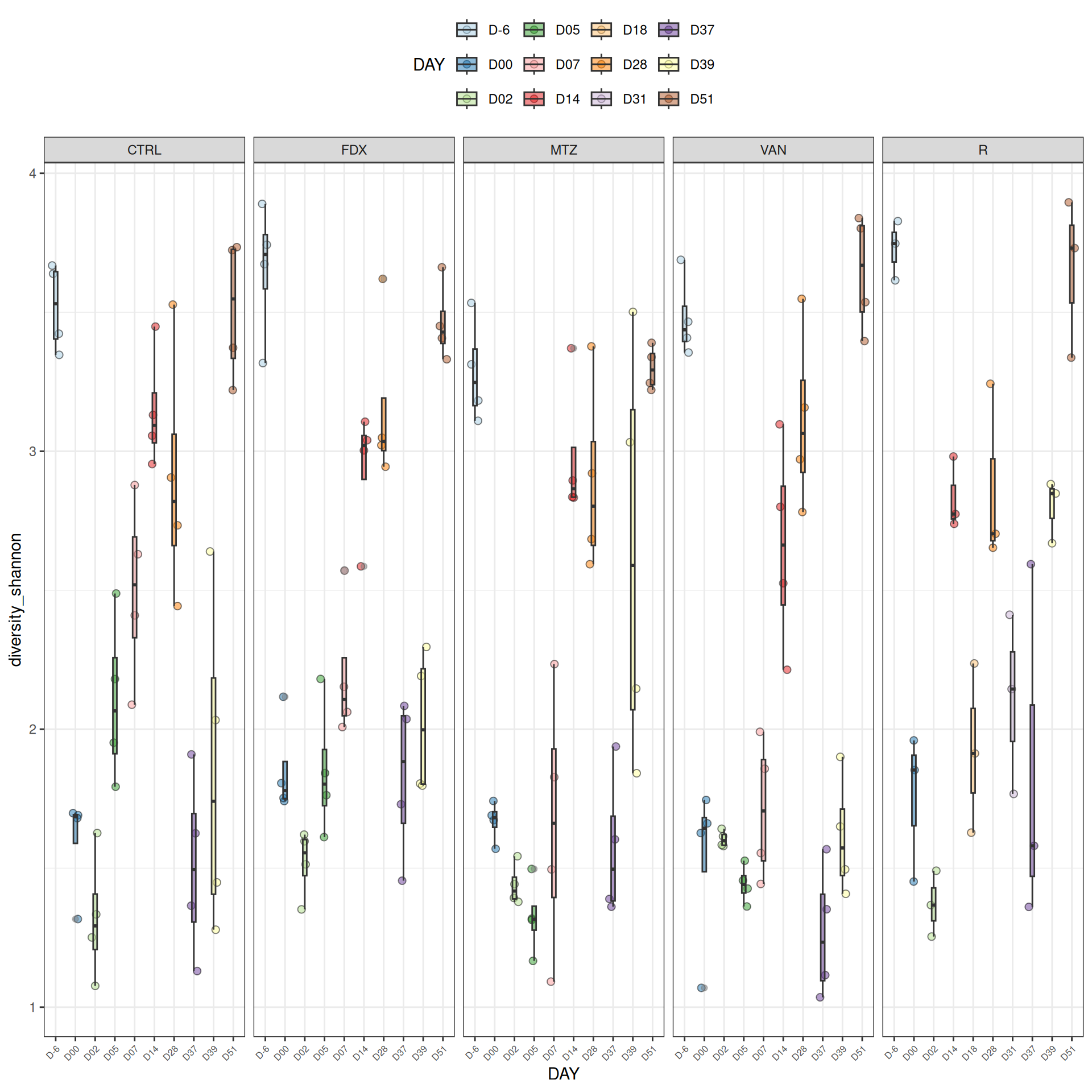
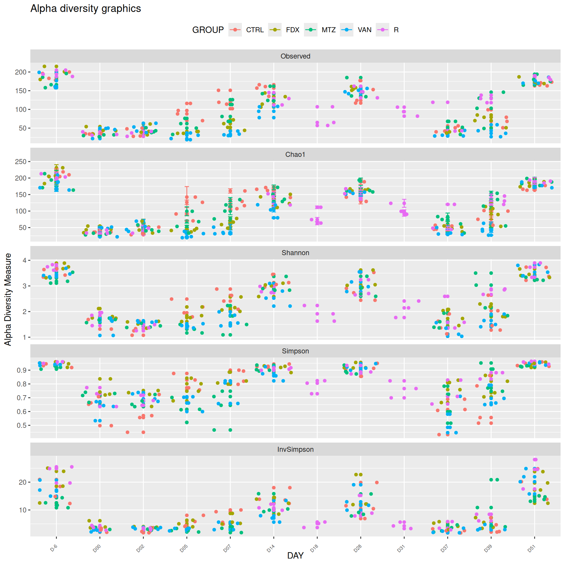
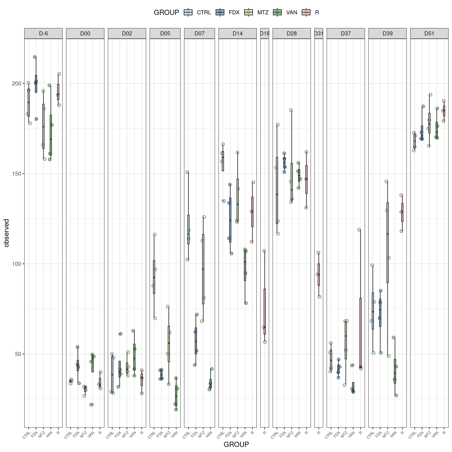
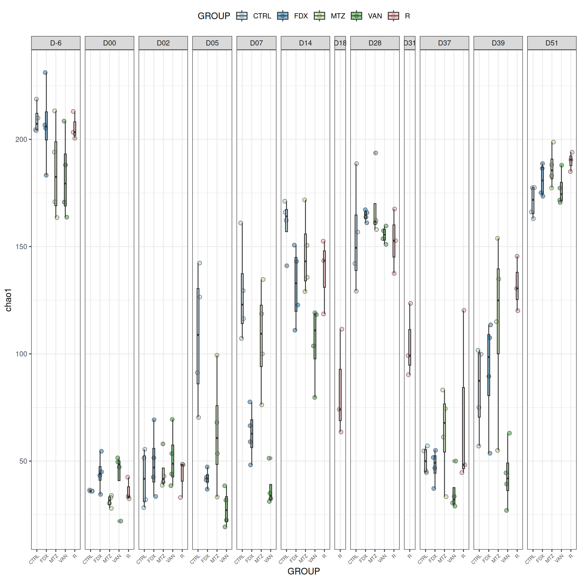
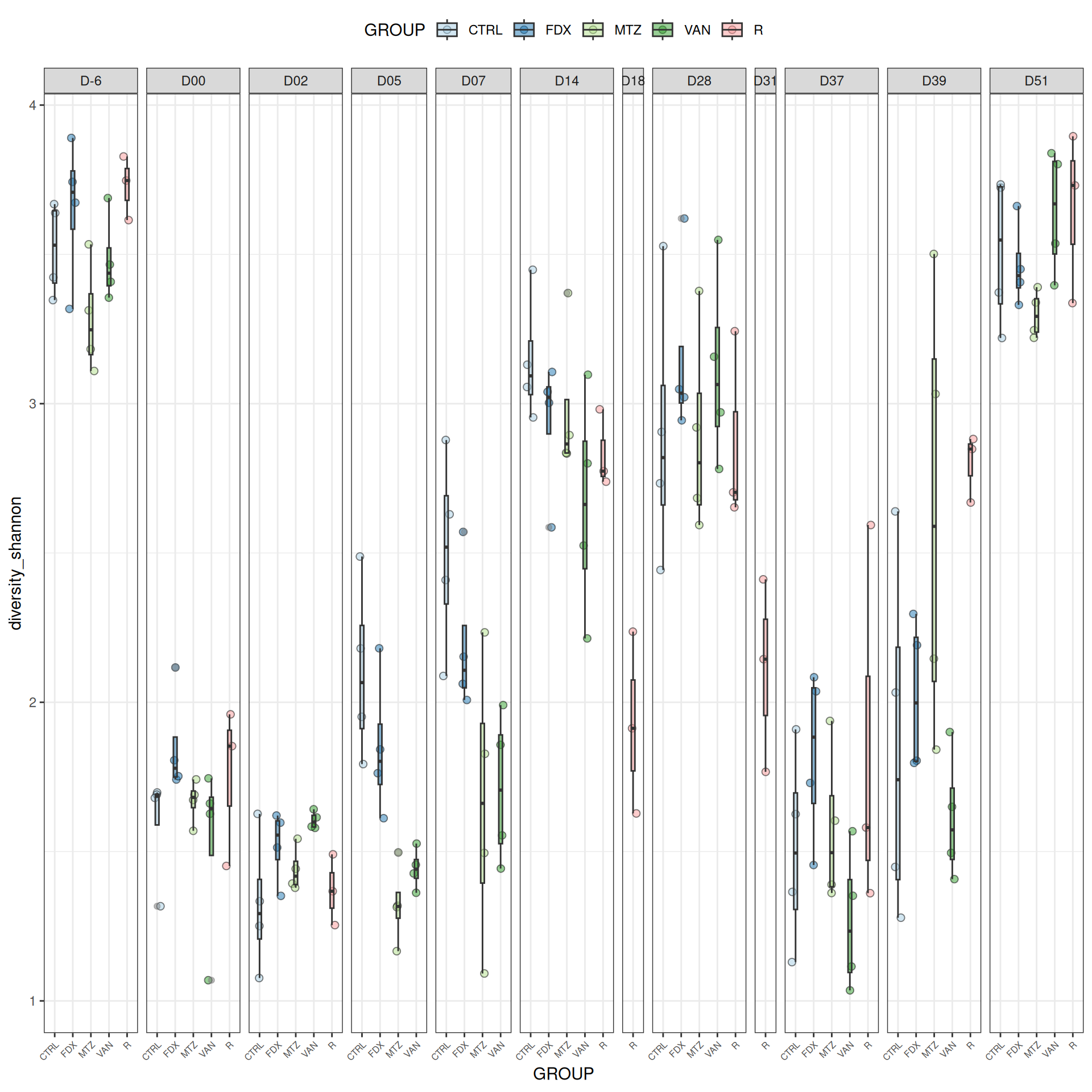
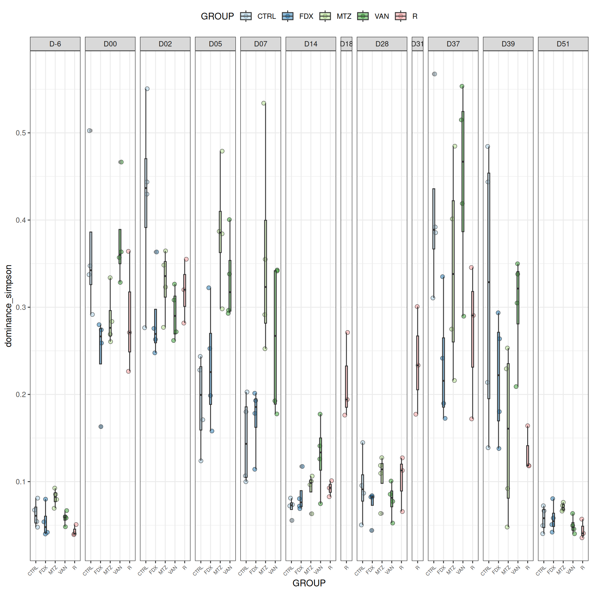
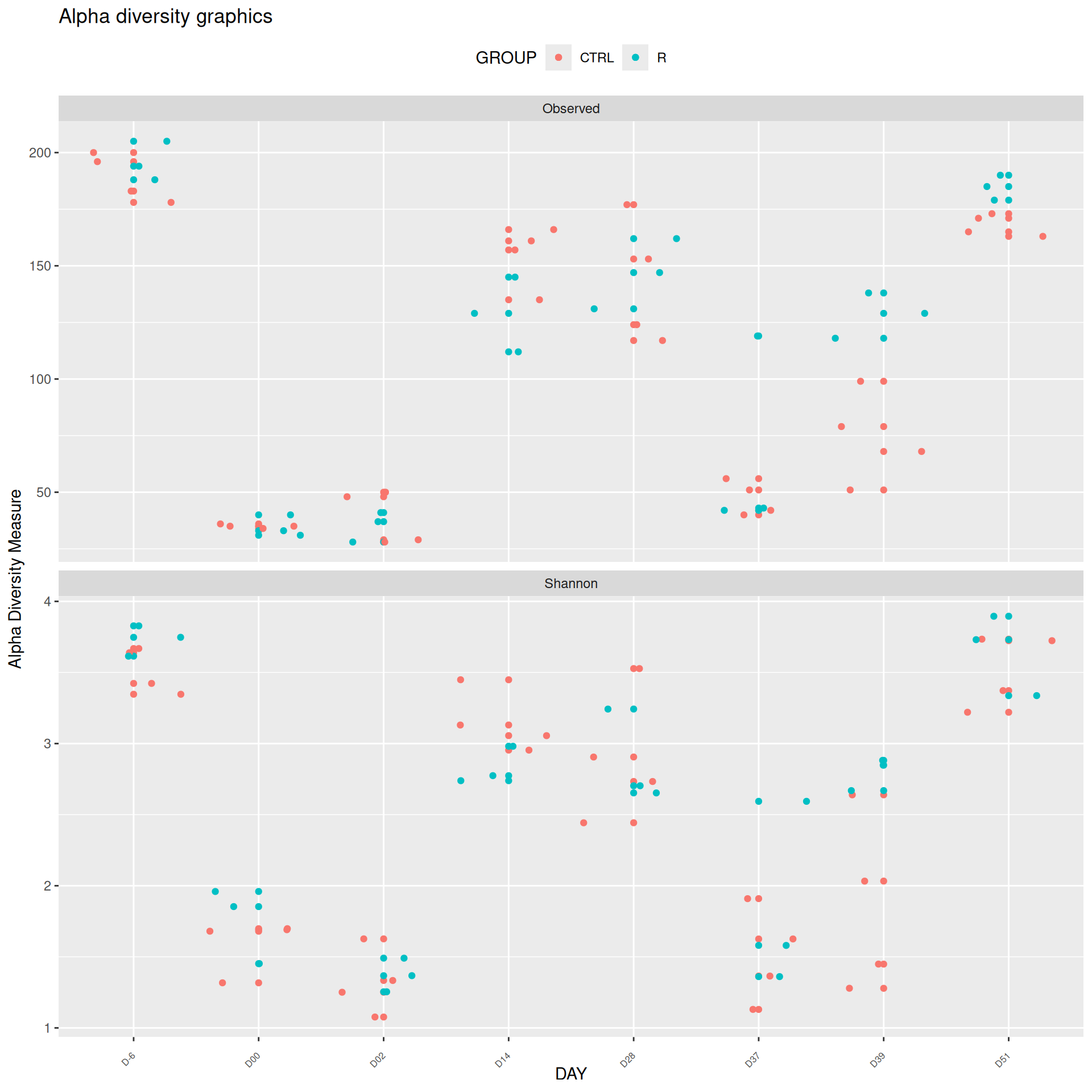
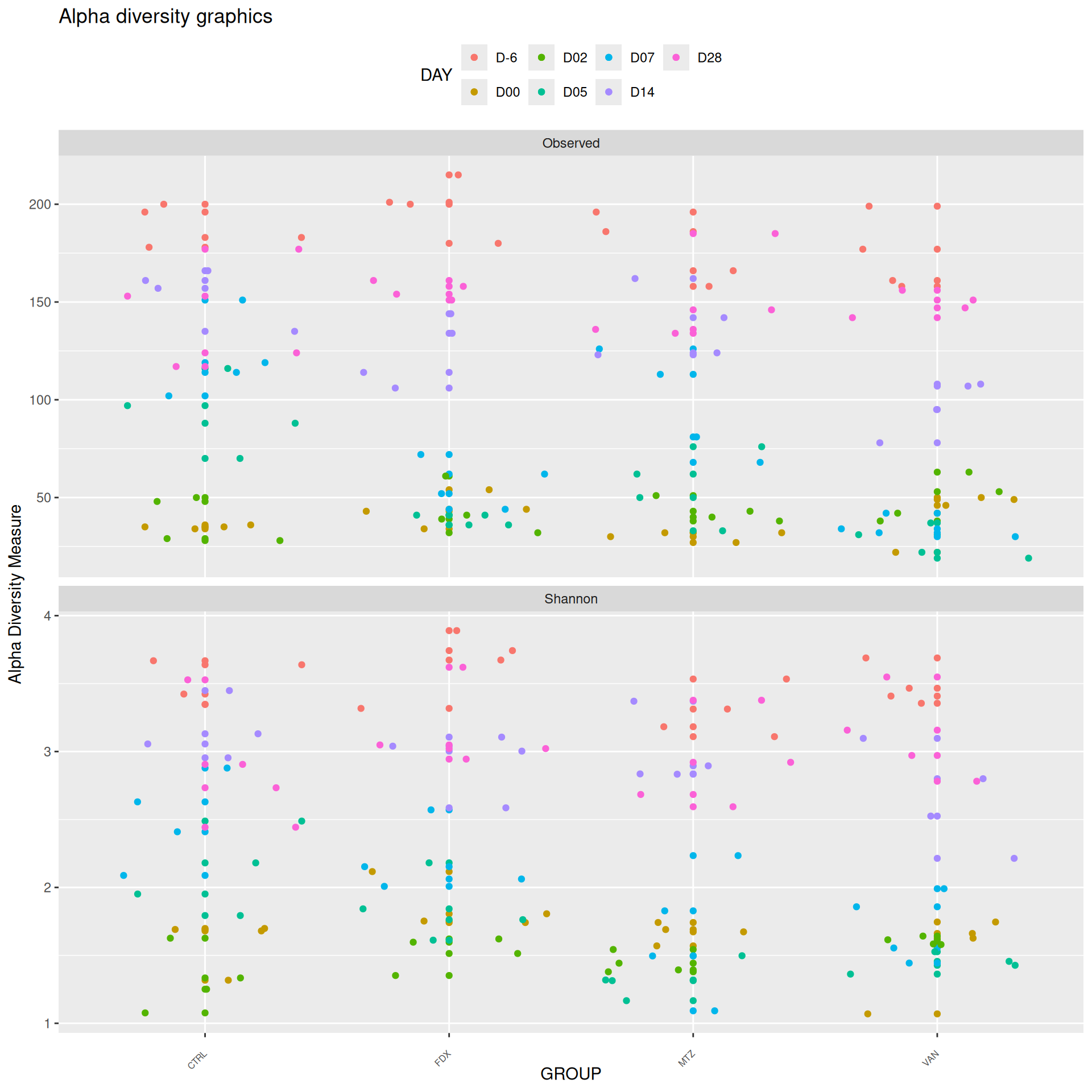
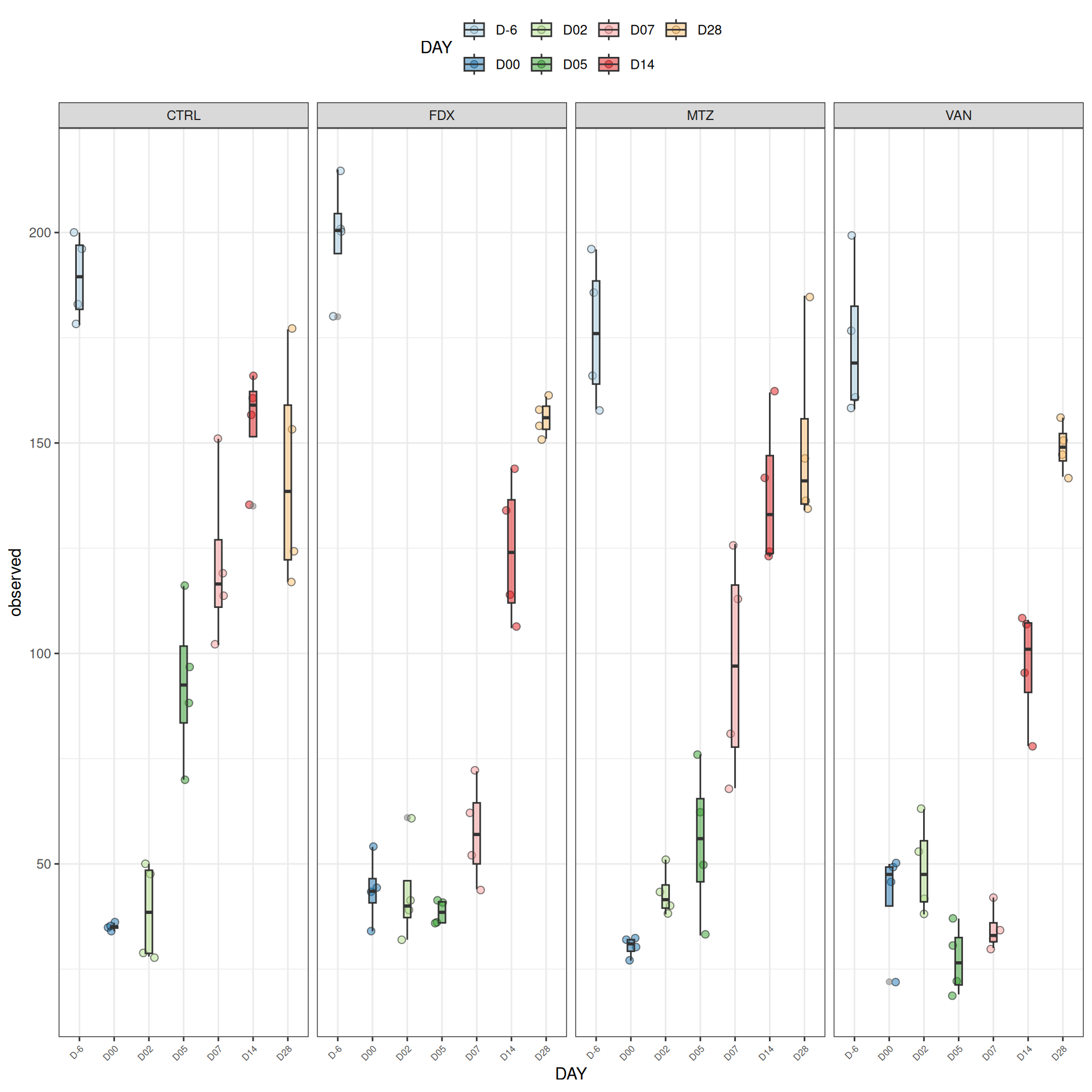
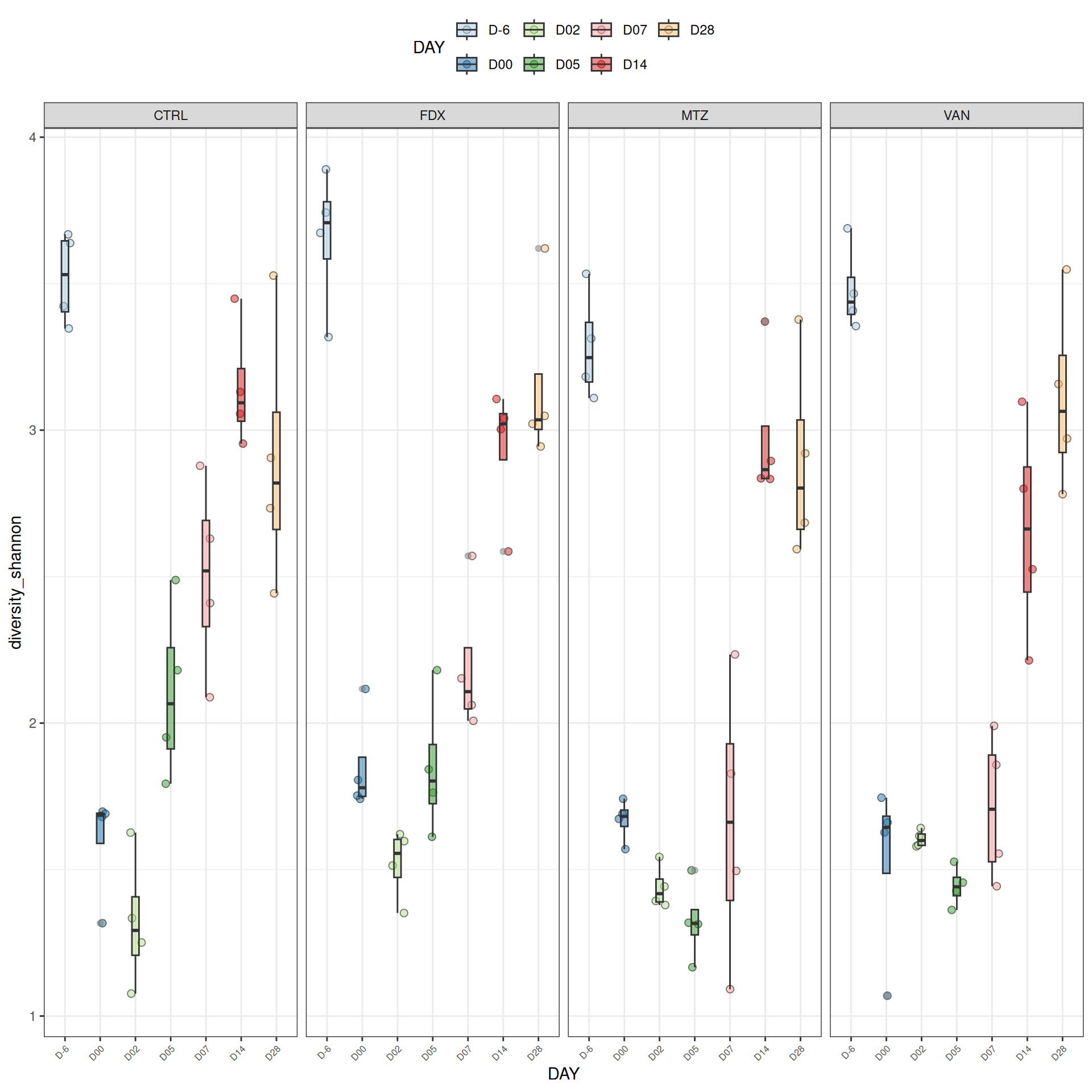
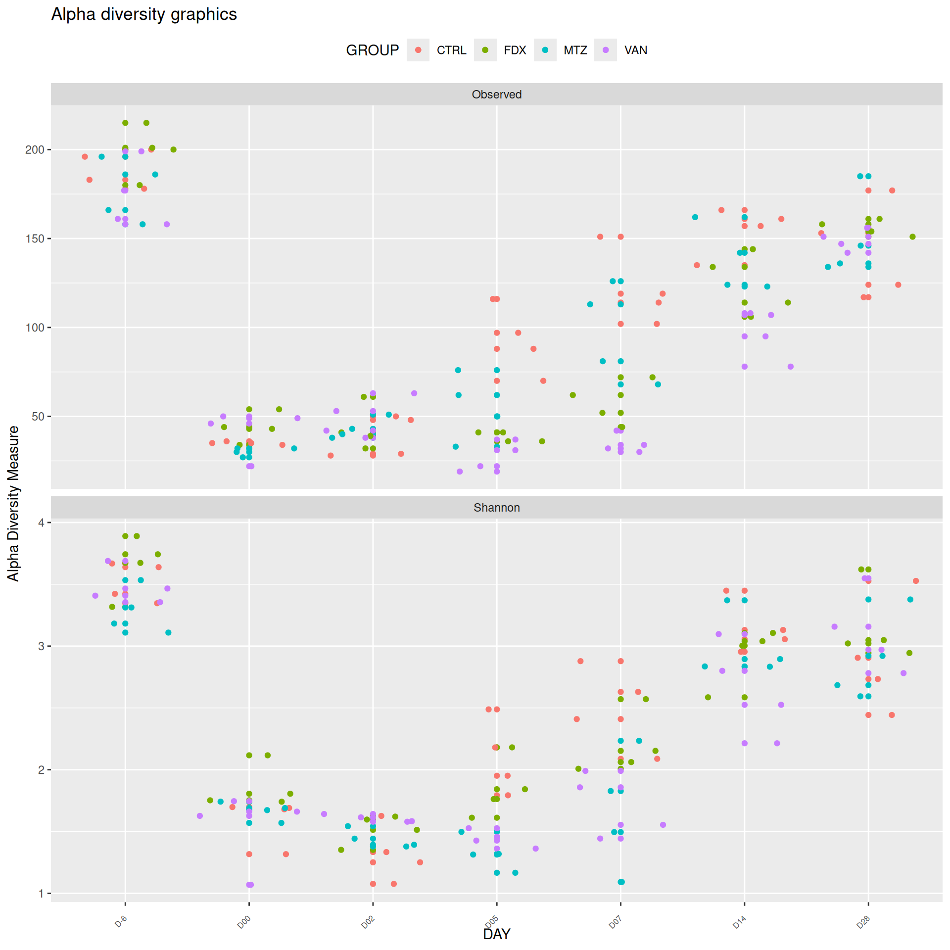
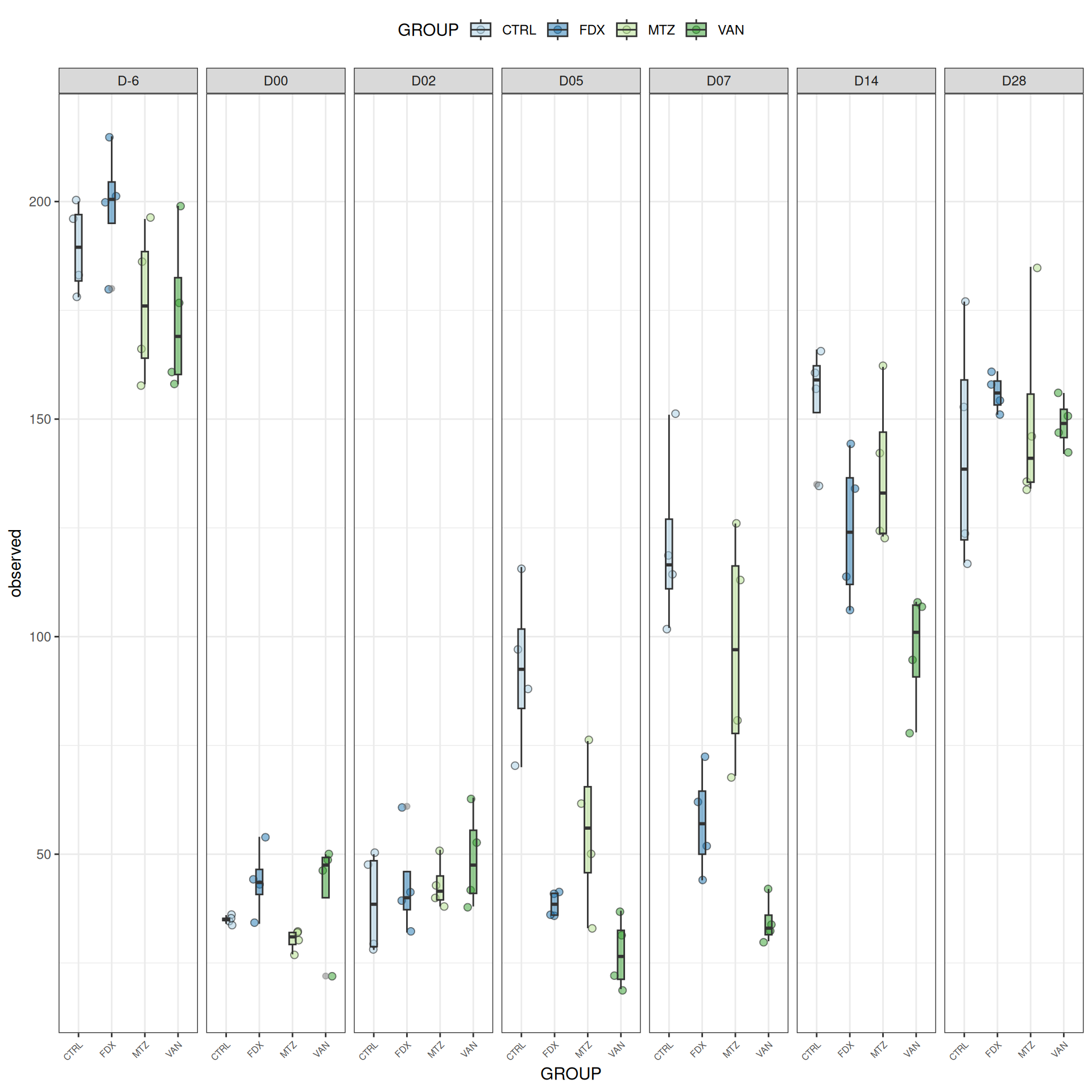
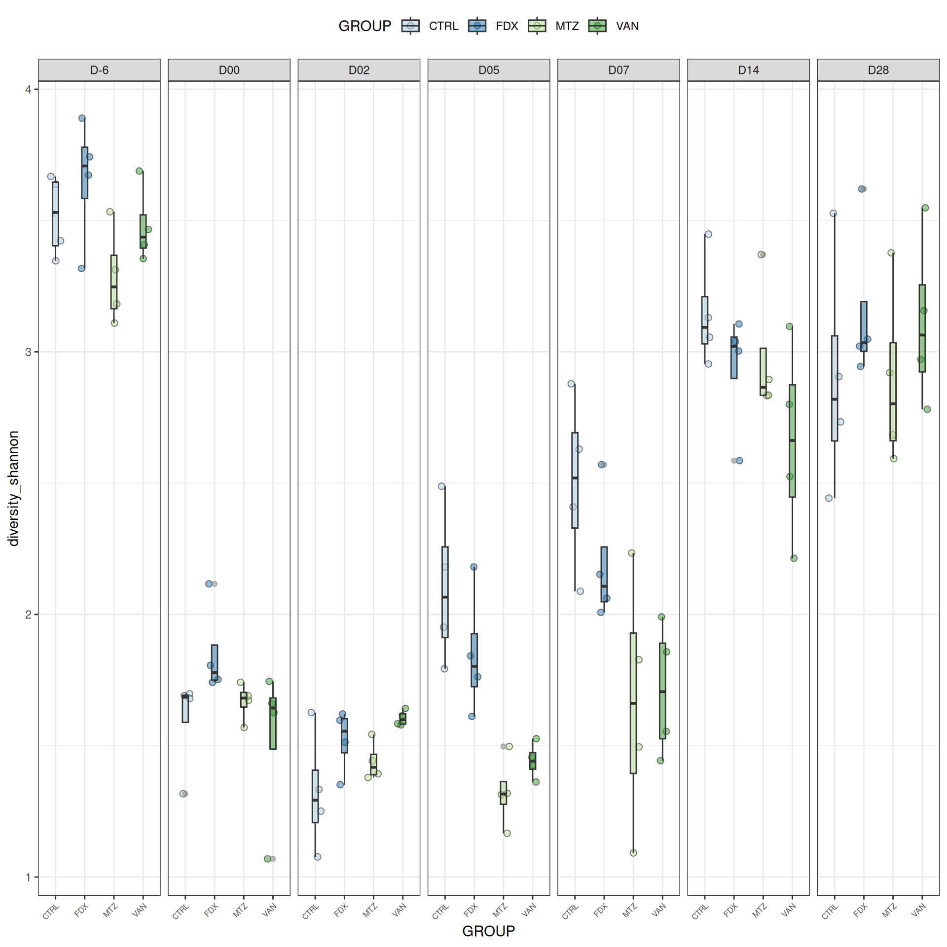
We observed that the alpha-diversity is mainly determined by DAY rather than GROUP. For each sample, the observed index measures the richness in the sample i.e. the total number of species in the community. Richness was highest in samples from J-6 and J51, and also J28 with more variability. It decreased on J00, J18 (GROUP R), J31 (GROUP R) and J37 on days of infection, and increased between infection dates. The other indices do not provide any additional information, as the trajectories are consistent with infection dates.
Alpha-diversity - statistical tests
We calculated the alpha-diversity indices and combined them with covariates from experimental design.
#model <- aov(Observed ~ DAY*GROUP, data = div_data)#anova(model)#coef(model)# produce parwise comparison test with Tukey's post-hoc correction #TukeyHSD(model, which ="DAY:GROUP")alphadiv.lm <-lm(Observed ~ DAY*GROUP, data = div_data)anova(alphadiv.lm)
Analysis of Variance Table

Response: Observed
           Df Sum Sq Mean Sq  F value    Pr(>F)
DAY        11 551807   50164 196.1617 < 2.2e-16 ***
GROUP       4  16254    4064  15.8902 9.536e-11 ***
DAY:GROUP  34  41407    1218   4.7623 2.426e-11 ***
Residuals 140  35802     256
---
Signif. codes:  0 '***' 0.001 '**' 0.01 '*' 0.05 '.' 0.1 ' ' 1
Show the code
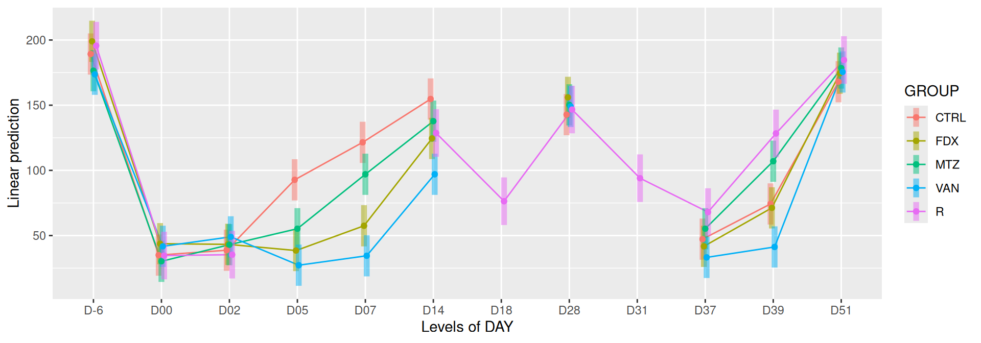
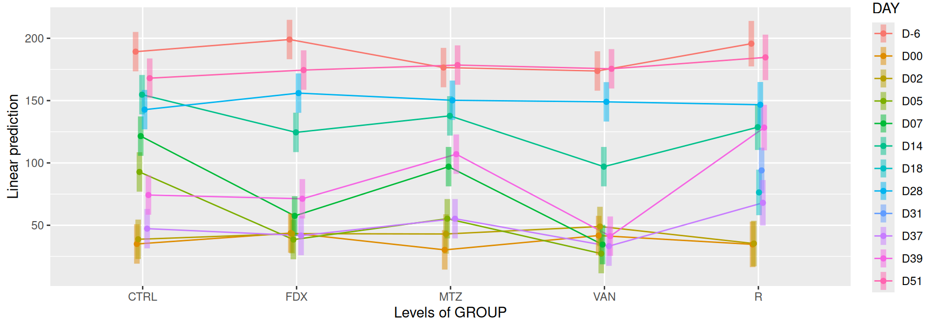
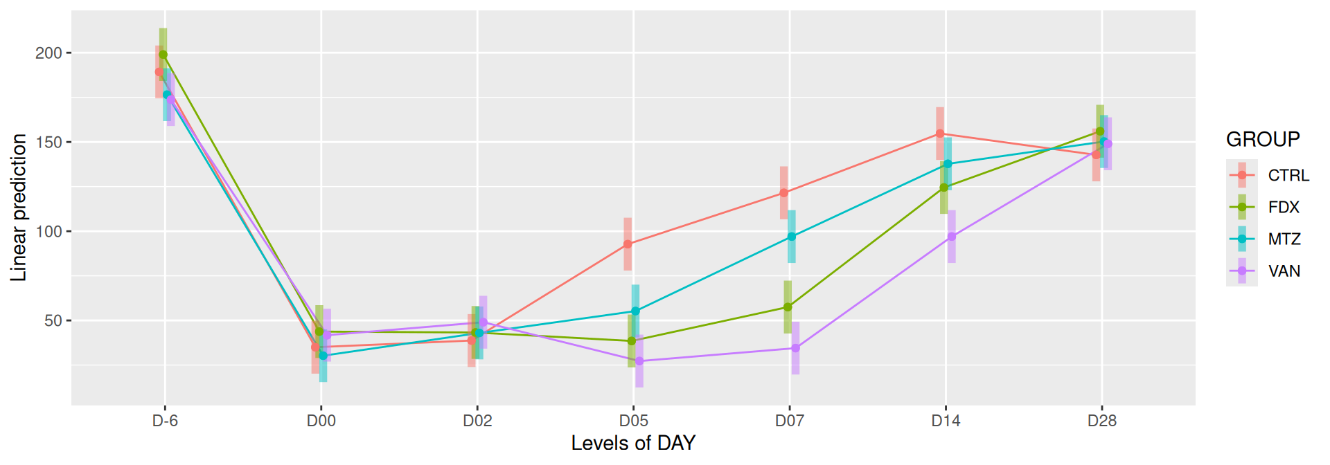
# interaction visualisationpar(mfrow =c(1,2))emmip(alphadiv.lm, GROUP ~ DAY, CIs =TRUE)
Show the code
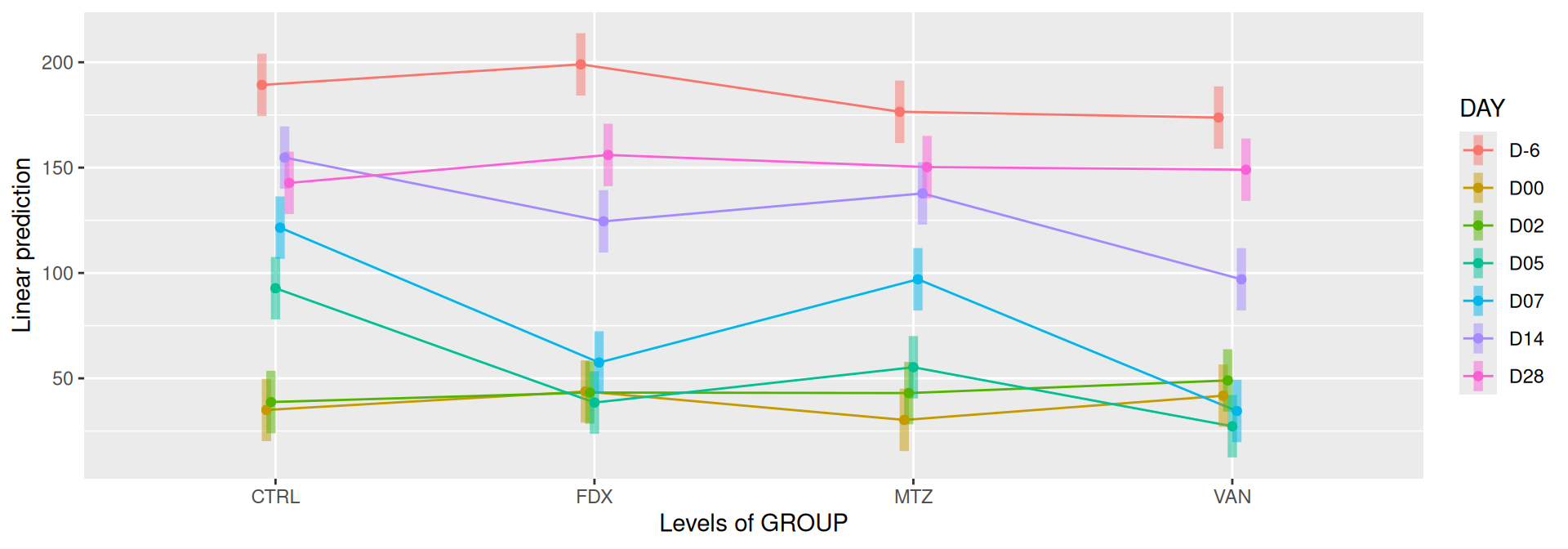
emmip(alphadiv.lm, DAY ~ GROUP, CIs =TRUE)
Show the code
par(mfrow =c(1,1))#tests EMM <-emmeans(alphadiv.lm, ~ DAY*GROUP)# tests correction are performed within the variable# P value adjustment: tukey method for comparing a family of 12 estimatescomp1 <-pairs(EMM, simple ="DAY")# P value adjustment: tukey method for comparing a family of 5 estimates comp2 <-pairs(EMM, simple ="GROUP")
Show the code
# P value adjustment: tukey method for comparing a family of 60 estimates res_emm <-contrast(EMM, method ="revpairwise", by =NULL, enhance.levels =c("DAY", "GROUP"), adjust ="tukey")
Important
Richness is significantly different by DAY, GROUP and also by the interaction DAY:GROUP. Pairwise tests between DAY, GROUP and also by the interaction DAY:GROUPwere performed with post hoc Tukey’s test to determine which were significant.
Beta-diversity
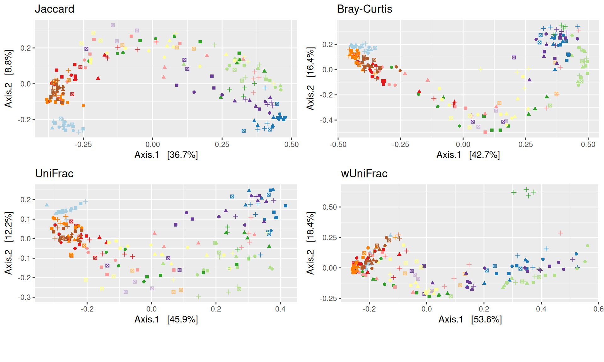
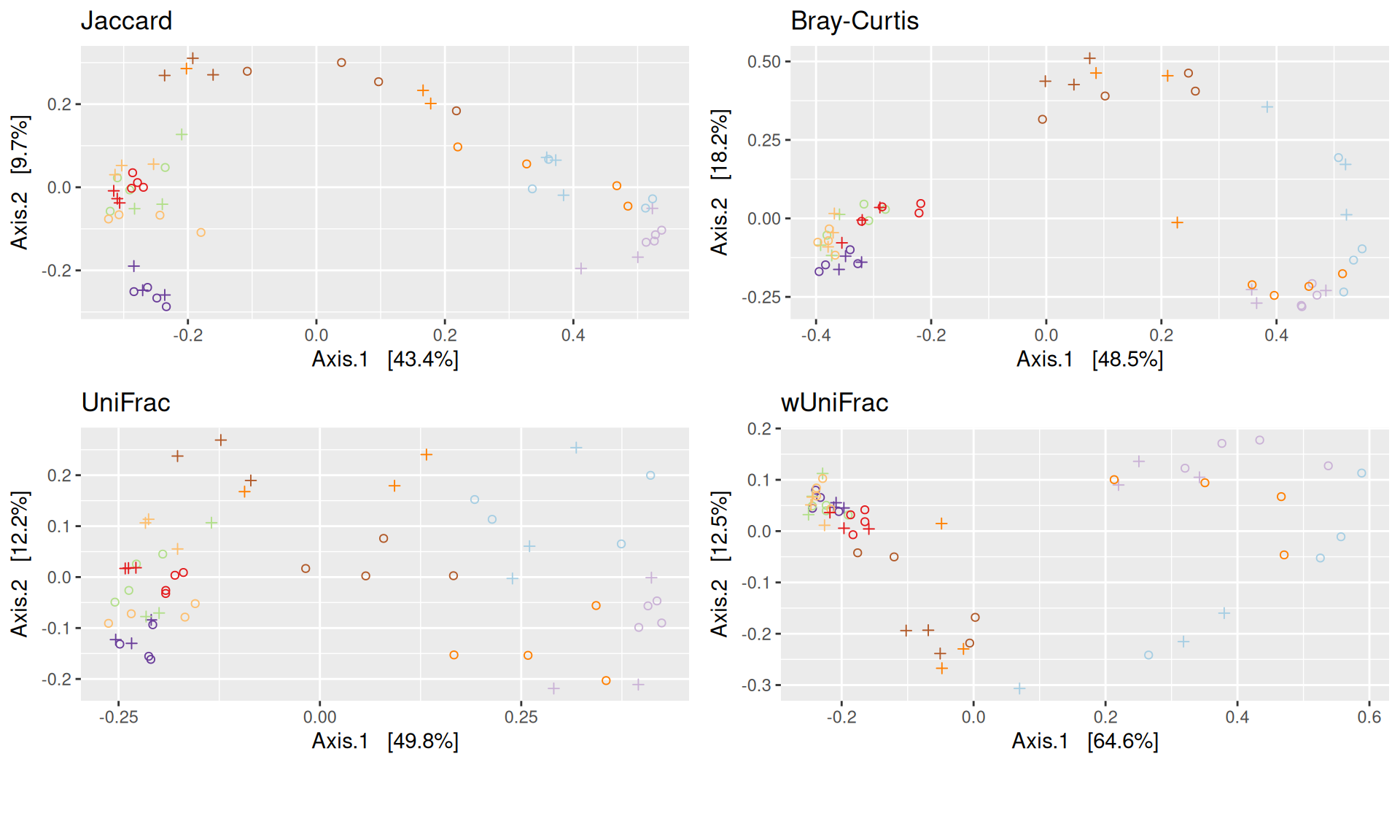
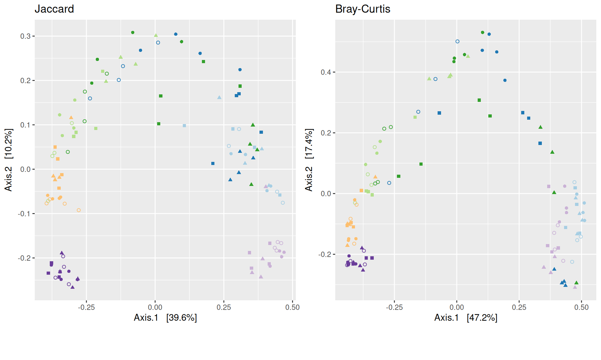
The dissimilarity between samples based on taxonomic composition is calculated with one of these Beta diversities: Bray-Curtis, Unweighted and weighted Unifrac, Jaccard index. The Jaccard index uses presence/absence information only whereas UniFrac integrates information from the phylogenetic tree.
The Multidimensional scaling (MDS / PCoA) showed that samples were distributed according to the variable DAY on the first two axes. Samples from J-6, J28 and J51 are homogeneous, close to each other and opposite to samples from J00 on the first axis. The others are distributed in both dimensions.
Permutation test for adonis under reduced model
Permutation: free
Number of permutations: 9999

vegan::adonis2(formula = dist.bc ~ DAY * GROUP, data = metadata, permutations = 9999)
          Df SumOfSqs      R2      F Pr(>F)
Model     49   44.616 0.81639 12.704  1e-04 ***
Residual 140   10.034 0.18361
Total    189   54.651 1.00000
---
Signif. codes:  0 '***' 0.001 '**' 0.01 '*' 0.05 '.' 0.1 ' ' 1
Show the code
# test with dist.jac, dist.uf, dist.wuf# model <- vegan::adonis2(dist.jac ~ DAY*GROUP, data = metadata, permutations = 9999)# print(model)
Important
The change in microbiota composition measured by the Bray-Curtis Beta diversity is significantly different between DAY, GROUP and also between the levels of the interaction factor DAY:GROUP at 0.05 significance level. The influence of the factors differs between ecosystems. Same results (not shown) with the other dissimilarities Jaccard, UniFrac, and wUniFrac were obtained.
Show the code
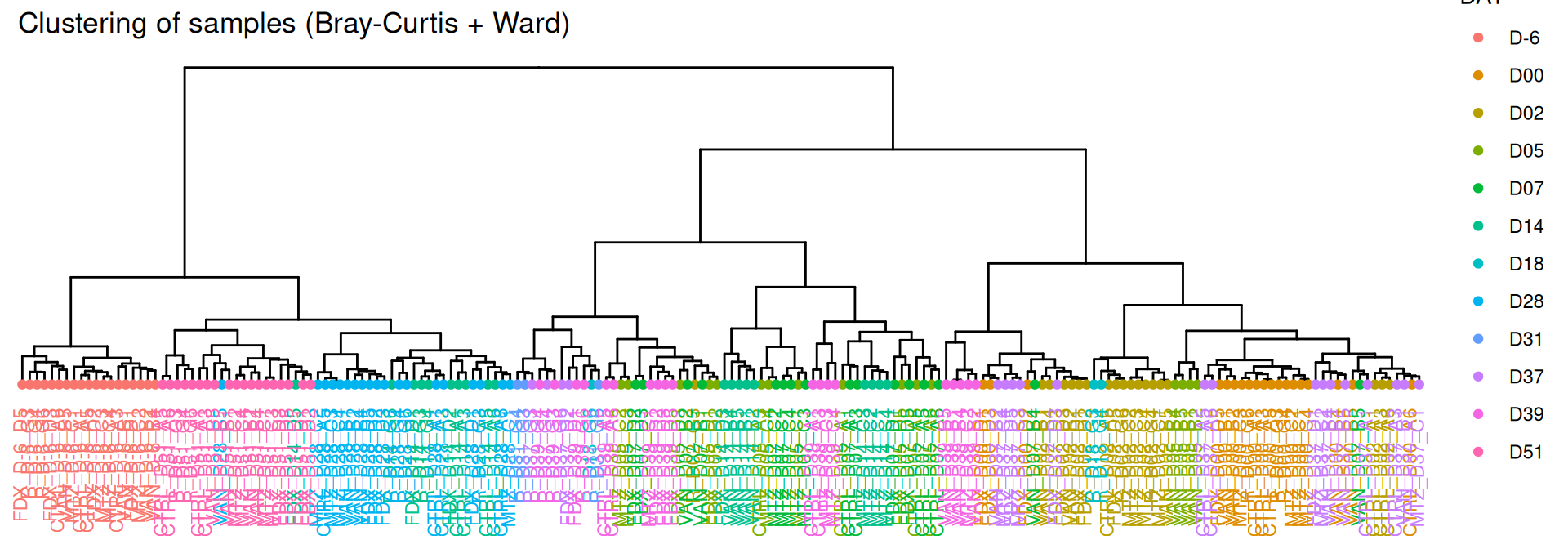
par(mar =c(3, 0, 2, 0), cex =0.6)phyloseq.extended::plot_clust(frogs_rare, dist ="bray", method ="ward.D2", color ="DAY",title ="Clustering of samples (Bray-Curtis + Ward)")
Important
Hierarchical clustering based on the Bray-Curtis dissimilarity and the Ward aggregation criterion shows that sample composition is not entirely structured by DAY. Groups were formed according to the date of infection and the existing DAY:GROUP interaction .
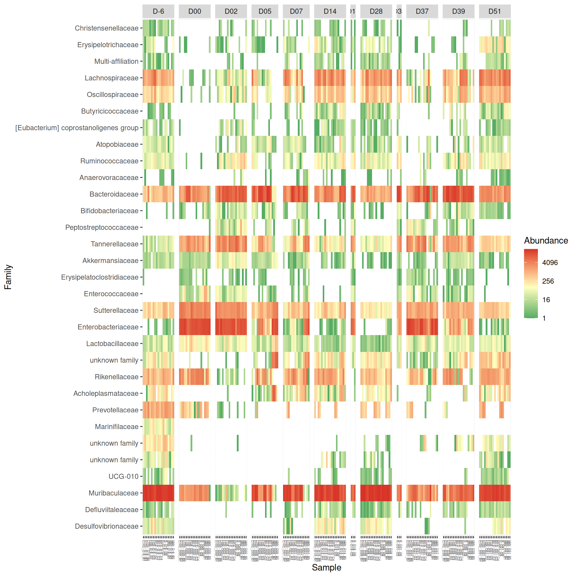
At Family and Genus taxonomic levels, we created heatmap plot using ordination methods to organize the rows.
# method = NULL if not ordinationp <- phyloseq::plot_heatmap(tax_glom(frogs_rare, taxrank="Family"), method ="NMDS",distance ="bray",sample.order="Label", # not ordination# taxa.order = "Family",taxa.label ="Family") +facet_grid(~ DAY, scales ="free_x", space ="free_x") +scale_fill_gradient2(low ="#1a9850", mid ="#ffffbf", high ="#d73027",na.value ="white", trans = scales::log_trans(4),midpoint =log(100, base =4))p
Show the code
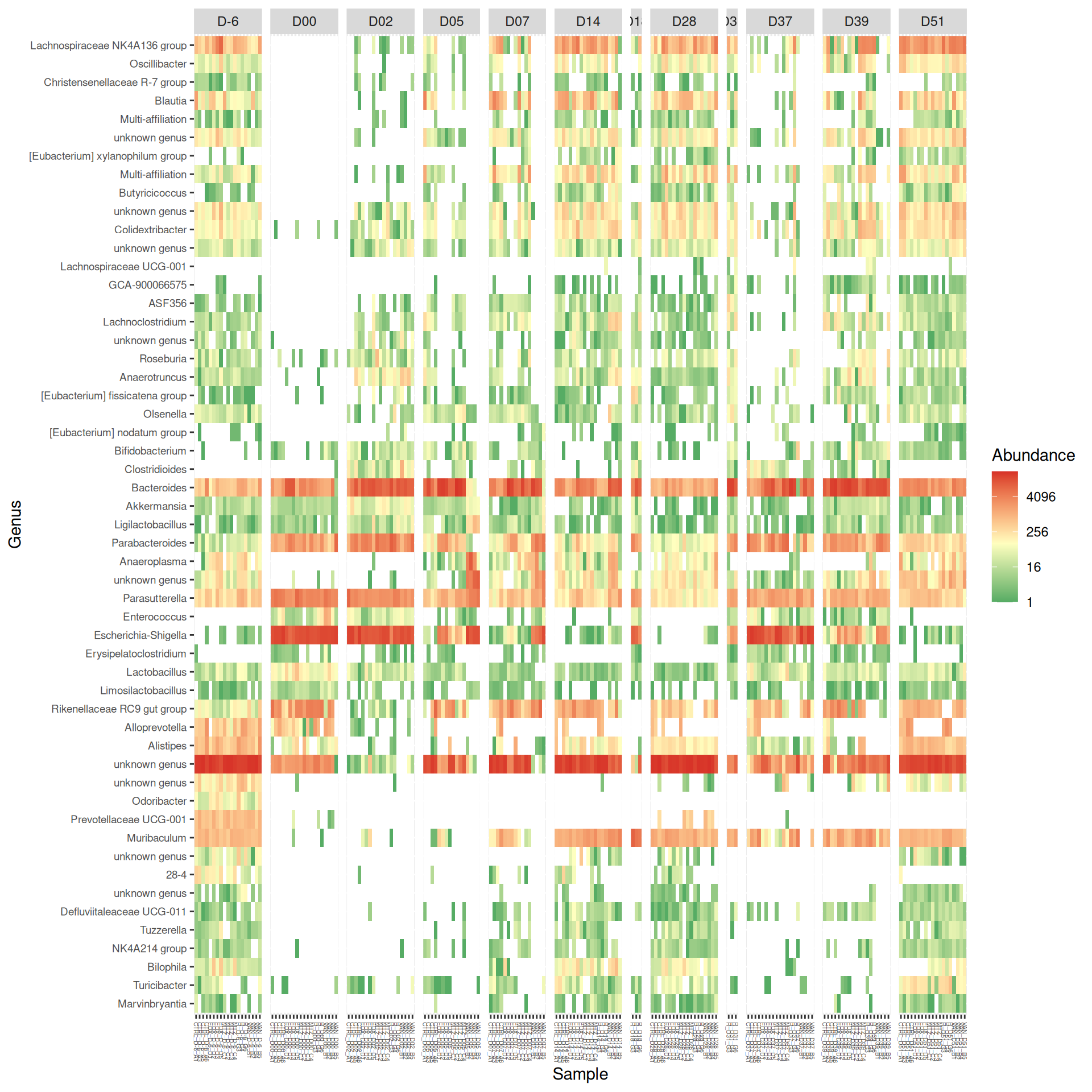
p <- phyloseq::plot_heatmap(tax_glom(frogs_rare, taxrank="Genus"), distance ="bray", method ="NMDS",sample.order="Label", # not ordination# taxa.order = "Family",taxa.label="Genus") +facet_grid(~ DAY, scales ="free_x", space ="free_x") +scale_fill_gradient2(low ="#1a9850", mid ="#ffffbf", high ="#d73027",na.value ="white", trans = scales::log_trans(4),midpoint =log(100, base =4))p
Important
As expected many bacteria disappeared at J00 due to antiobitics. Clostridoides was absent at J-6, J00, J28 and J51. It was present at J02 and J37, and partially present during the evolution of the infection. Abundance profiles appeared fairly similar similar at J-6, J00, J28 and J51. We observed differences for Bifidobacterium, 28-4, Oscillibacter, and Prevotellaceae UCG-001.
Annex1: study on subset including only R and CTRL treatments
Important
Note that the rarefaction was performed on all samples from the complete study. We extracted samples of interest from the frogs_rare phyloseq object to calculate alpha diversity. Alpha diversity is calculated within sample and do not change with the previous analyses on the complete study.
Show the code
frogs_rare_withR <-subset_samples(frogs_rare, DAY %in%c("D-6", "D00", "D02", "D14", "D28", "D37", "D39", "D51") & GROUP %in%c("R", "CTRL"))
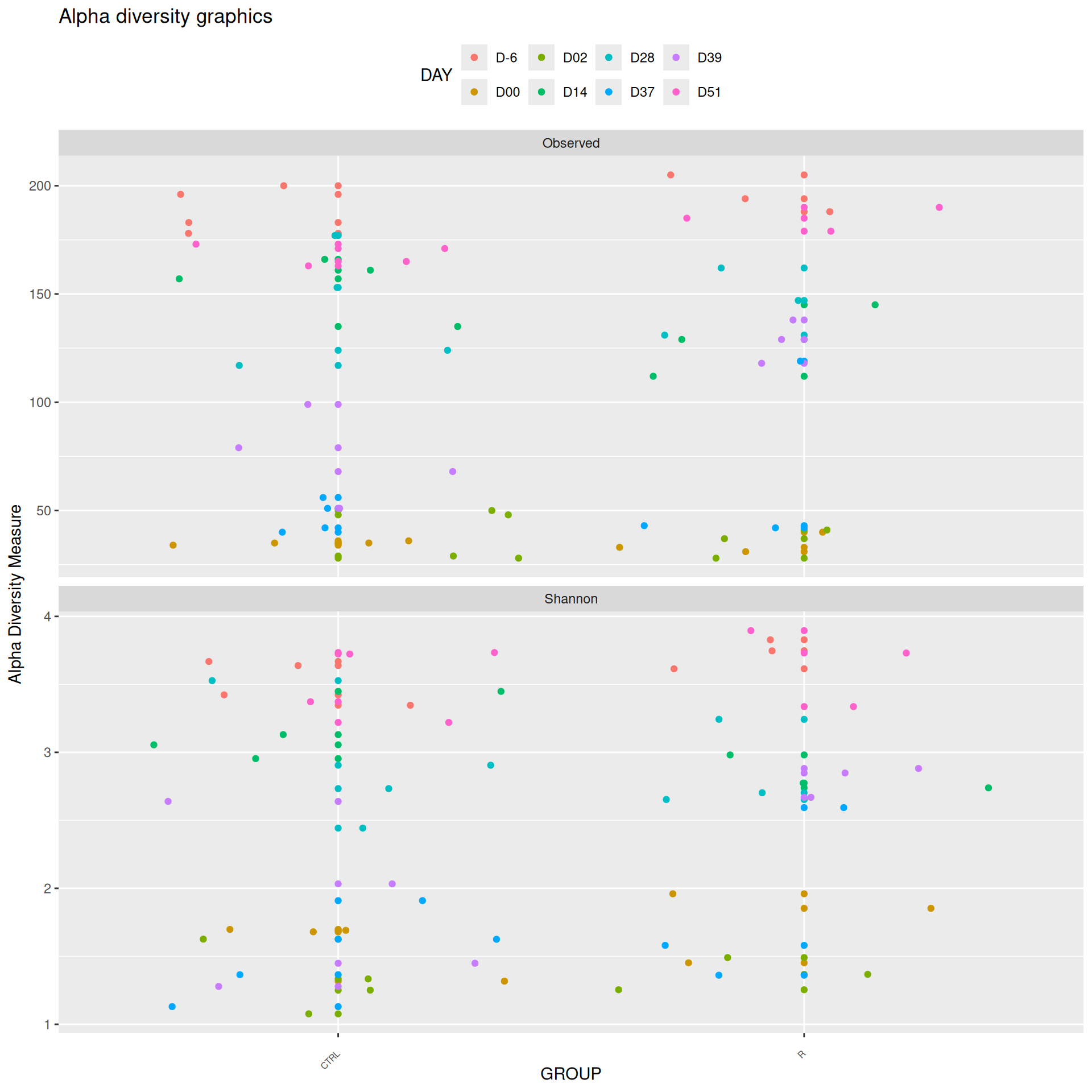
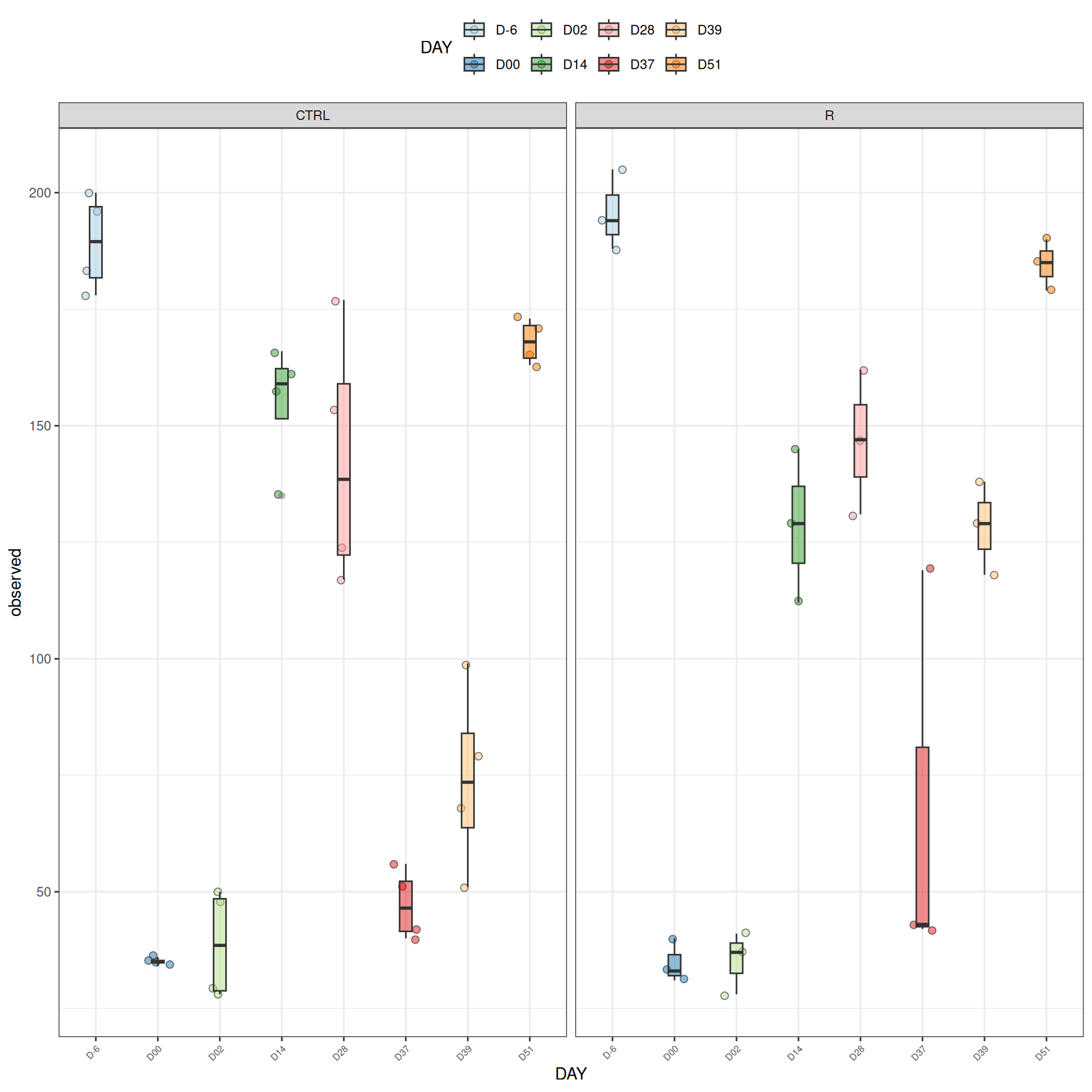
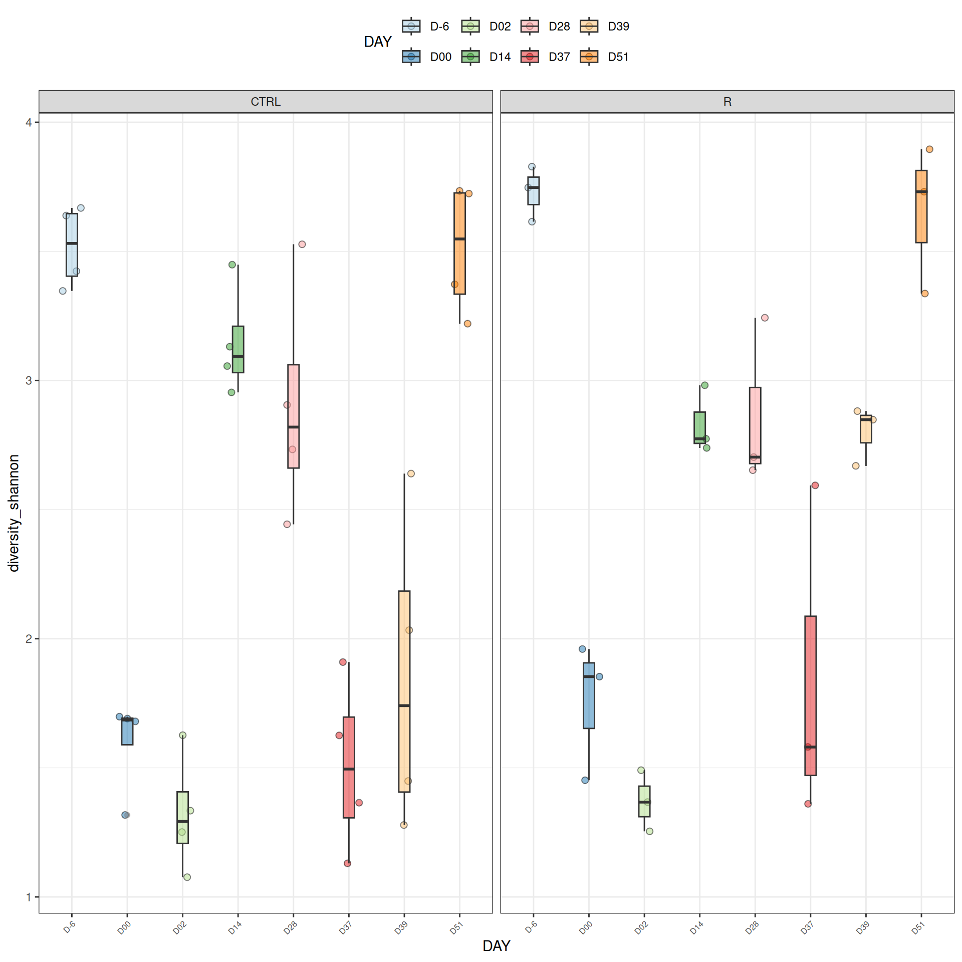
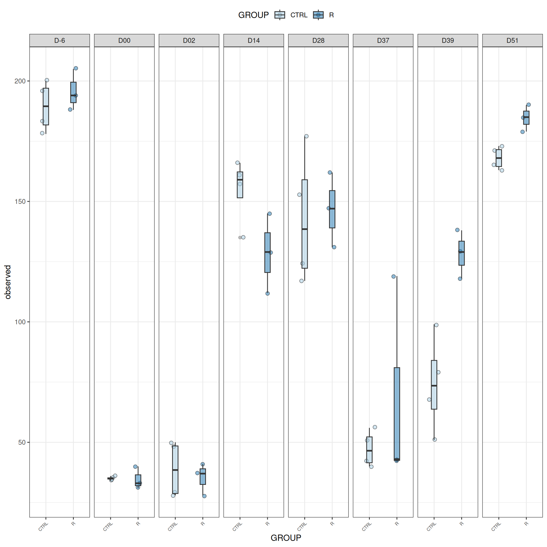
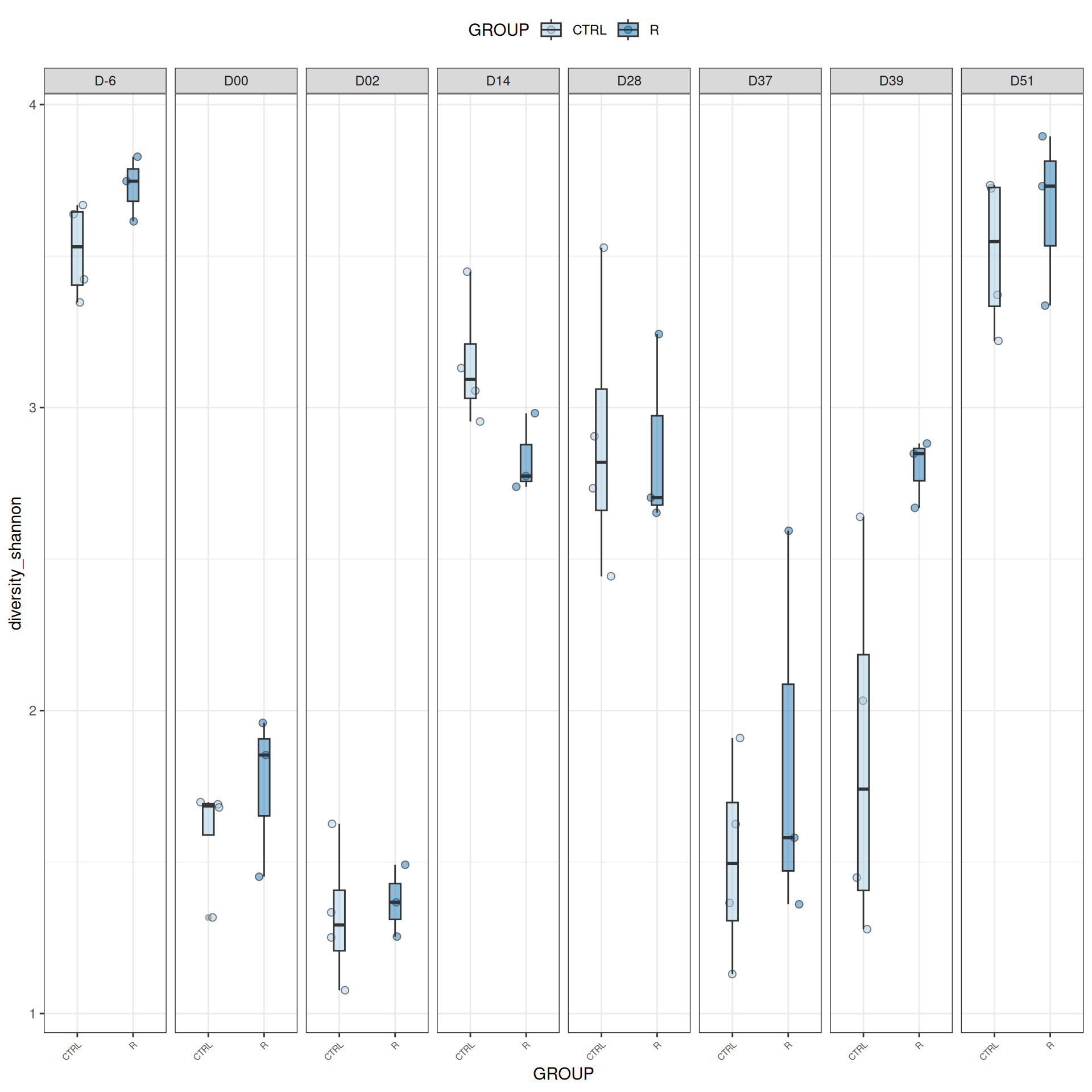
We observed that the alpha-diversity is mainly determined by DAY rather than GROUP. For each sample, the observed index measures the richness in the sample i.e. the total number of species in the community. Richness was highest in samples from J-6 and J51, and also J28 with more variability. It decreased on J00, J18 (GROUP R), J31 (GROUP R) and J37 on days of infection, and increased between infection dates. The other indices do not provide any additional information, as the trajectories are consistent with infection dates.
Alpha-diversity - statistical tests
We calculated the alpha-diversity indices and combined them with covariates from experimental design.
#model <- aov(Observed ~ DAY*GROUP, data = div_data)#anova(model)#coef(model)# produce parwise comparison test with Tukey's post-hoc correction #TukeyHSD(model, which ="DAY:GROUP")alphadiv.lm <-lm(Observed ~ DAY*GROUP, data = div_data)anova(alphadiv.lm)
Analysis of Variance Table

Response: Observed
          Df Sum Sq Mean Sq  F value    Pr(>F)
DAY        7 190906 27272.3 103.6067 < 2.2e-16 ***
GROUP      1   1111  1110.9   4.2201  0.046522 *
DAY:GROUP  7   6401   914.4   3.4740  0.005321 **
Residuals 40  10529   263.2
---
Signif. codes:  0 '***' 0.001 '**' 0.01 '*' 0.05 '.' 0.1 ' ' 1
Show the code
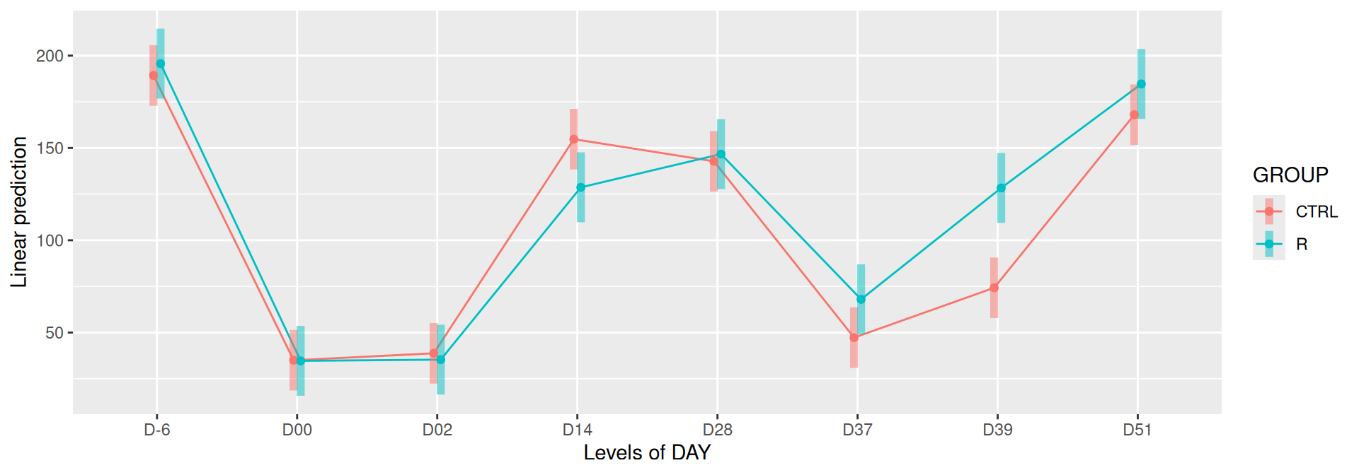
# interaction visualisationpar(mfrow =c(1,2))emmip(alphadiv.lm, GROUP ~ DAY, CIs =TRUE)
Show the code
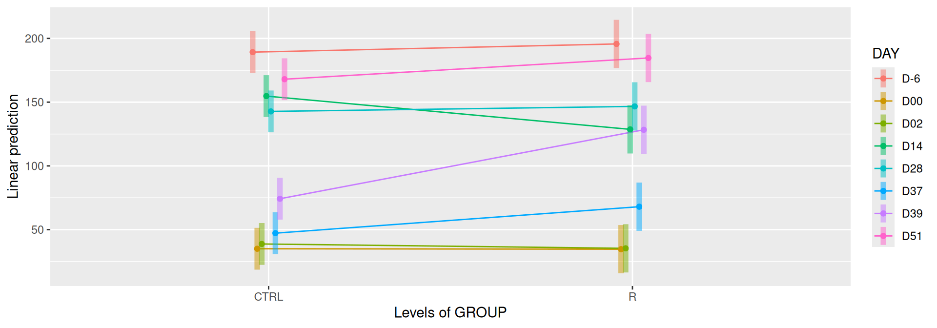
emmip(alphadiv.lm, DAY ~ GROUP, CIs =TRUE)
Show the code
par(mfrow =c(1,1))#tests EMM <-emmeans(alphadiv.lm, ~ DAY*GROUP)# tests correction are performed within the variable# P value adjustment: tukey method for comparing a family of 12 estimatescomp1 <-pairs(EMM, simple ="DAY")# P value adjustment: tukey method for comparing a family of 5 estimates comp2 <-pairs(EMM, simple ="GROUP")
Show the code
# P value adjustment: tukey method for comparing a family of 60 estimates res_emm <-contrast(EMM, method ="revpairwise", by =NULL, enhance.levels =c("DAY", "GROUP"), adjust ="tukey")
Important
Richness is significantly different by DAY, GROUP and also by the interaction DAY:GROUP. Pairwise tests between DAY, GROUP and also by the interaction DAY:GROUPwere performed with post hoc Tukey’s test to determine which were significant.
Beta-diversity with R and CTRL treatments
The dissimilarity between samples based on taxonomic composition is calculated with one of these Beta diversities: Bray-Curtis, Unweighted and weighted Unifrac, Jaccard index. The Jaccard index uses presence/absence information only whereas UniFrac integrates information from the phylogenetic tree.
Show the code
# use all samples from the complete study frogs_raredist.jac <- phyloseq::distance(frogs_rare, method ="cc")dist.bc <- phyloseq::distance(frogs_rare, method ="bray")dist.uf <- phyloseq::distance(frogs_rare, method ="unifrac")dist.wuf <- phyloseq::distance(frogs_rare, method ="wunifrac")distance_list <-list("Jaccard"= dist.jac,"Bray-Curtis"= dist.bc,"UniFrac"= dist.uf,"wUniFrac"= dist.wuf)
# Mahendra's function# used own color's palette and shapemy_pcoa_with_arrows2 <-function(physeq = mydata_rare, variable1, variable2, shapeval, colorpal) {# select samples of interest where all samples were used to calculate the distances between samples # dist.jac is previously calculated with all samples of the study#dist.c <- phyloseq::distance(physeq, "jaccard") dist.c <- dist.jac %>%as.matrix() %>%`[`(sample_names(physeq), sample_names(physeq)) %>%as.dist() ord.c <-ordinate(physeq, "MDS", dist.c) p <-plot_ordination(physeq, ord.c)# ## Build arrow data plot_data <- p$data arrow_data <- plot_data %>%group_by(pick({{variable2}}, {{variable1}})) %>%arrange({{variable1}}) %>%mutate(xend = Axis.1, xstart =lag(xend),yend = Axis.2, ystart =lag(yend) )## Plot with arrows p +aes(shape = .data[[ variable2 ]], color = .data[[ variable1 ]]) +scale_shape_manual(values = shapeval) +scale_color_manual(name = colorpal$name,labels = colorpal$labels,values = colorpal$values) +theme_bw() +geom_segment(data = arrow_data,aes(x = xstart, y = ystart, xend = xend, yend = yend),size =0.8, linetype ="3131",arrow =arrow(length=unit(0.1,"inches")),show.legend =FALSE) +geom_point(size =3) +theme(legend.position ="bottom")}
Show the code
# MDS plot for samples of interests # from distance calculated with all samples of the complete study# used https://colorbrewer2.org/#type=qualitative&scheme=Paired&n=12Jour_pal <-list(name ="DAY",labels =c("D-6", "D00", "D02", "D14", "D28", "D37", "D39", "D51"),values =c("#6a3d9a", "#cab2d6", "#a6cee3", "#b2df8a", "#fdbf6f", "#ff7f00", "#b15928", "#e31a1c"))GROUP_shape <-list(values =c(1, 3))my_plot2(variable1 ="DAY",variable2 ="GROUP",physeq = frogs_rare_withR,shapeval = GROUP_shape$values,colorpal = Jour_pal )
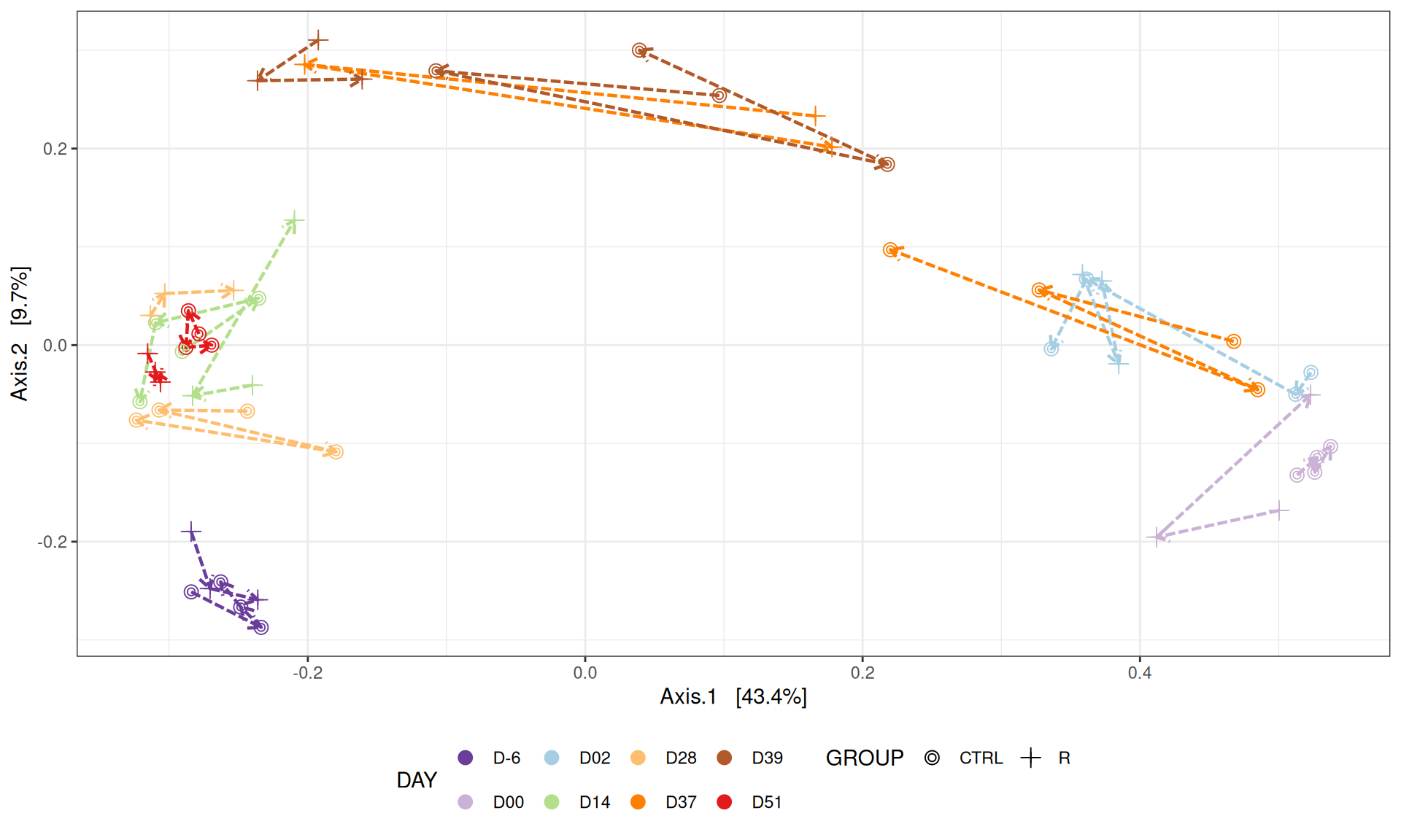
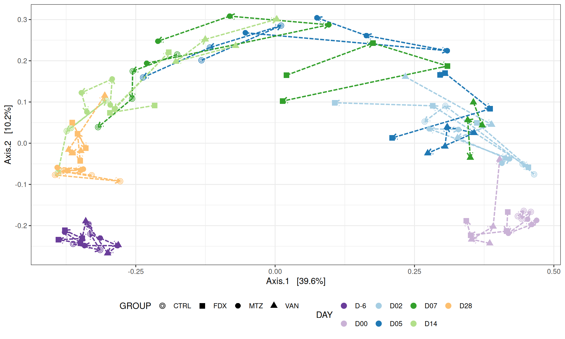
We use the Jaccard distance and show MDS trajectories of the communities intra conditions.
Show the code
# MDS plot for samples of interests # from distance calculated with all samples of the complete study# used https://colorbrewer2.org/#type=qualitative&scheme=Paired&n=12p <-my_pcoa_with_arrows2(variable1 ="DAY",variable2 ="GROUP",physeq = frogs_rare_withR,shapeval = GROUP_shape$values,colorpal = Jour_pal)p
Important
The Multidimensional scaling (MDS / PCoA) showed that samples were distributed according to the variable DAY on the first two axes. Samples from J-6, J28 and J51 are homogeneous, close to each other and opposite to samples from J00 on the first axis. The others are distributed in both dimensions.
Permutation test for adonis under reduced model
Permutation: free
Number of permutations: 9999

vegan::adonis2(formula = dist.bc ~ DAY * GROUP, data = metadata, permutations = 9999)
         Df SumOfSqs      R2      F Pr(>F)
Model    15  12.8691 0.83797 13.792  1e-04 ***
Residual 40   2.4883 0.16203
Total    55  15.3574 1.00000
---
Signif. codes:  0 '***' 0.001 '**' 0.01 '*' 0.05 '.' 0.1 ' ' 1
Important
The change in microbiota composition measured by the Bray-Curtis Beta diversity is significantly different between DAY, GROUP and also between the levels of the interaction factor DAY:GROUP at 0.05 significance level. The influence of the factors differs between ecosystems.
Annex2: study on subset excluding R treatment
Important
Note that the rarefaction was performed on all samples from the complete study. We extracted samples of interest from the frogs_rare phyloseq object to calculate alpha diversity. Alpha diversity is calculated within sample and do not change with the previous analyses on the complete study.
Show the code
frogs_rare_withoutR <-subset_samples(frogs_rare, GROUP !="R"& DAY %in%c("D-6","D00","D02","D05","D07","D14","D18","D28"))
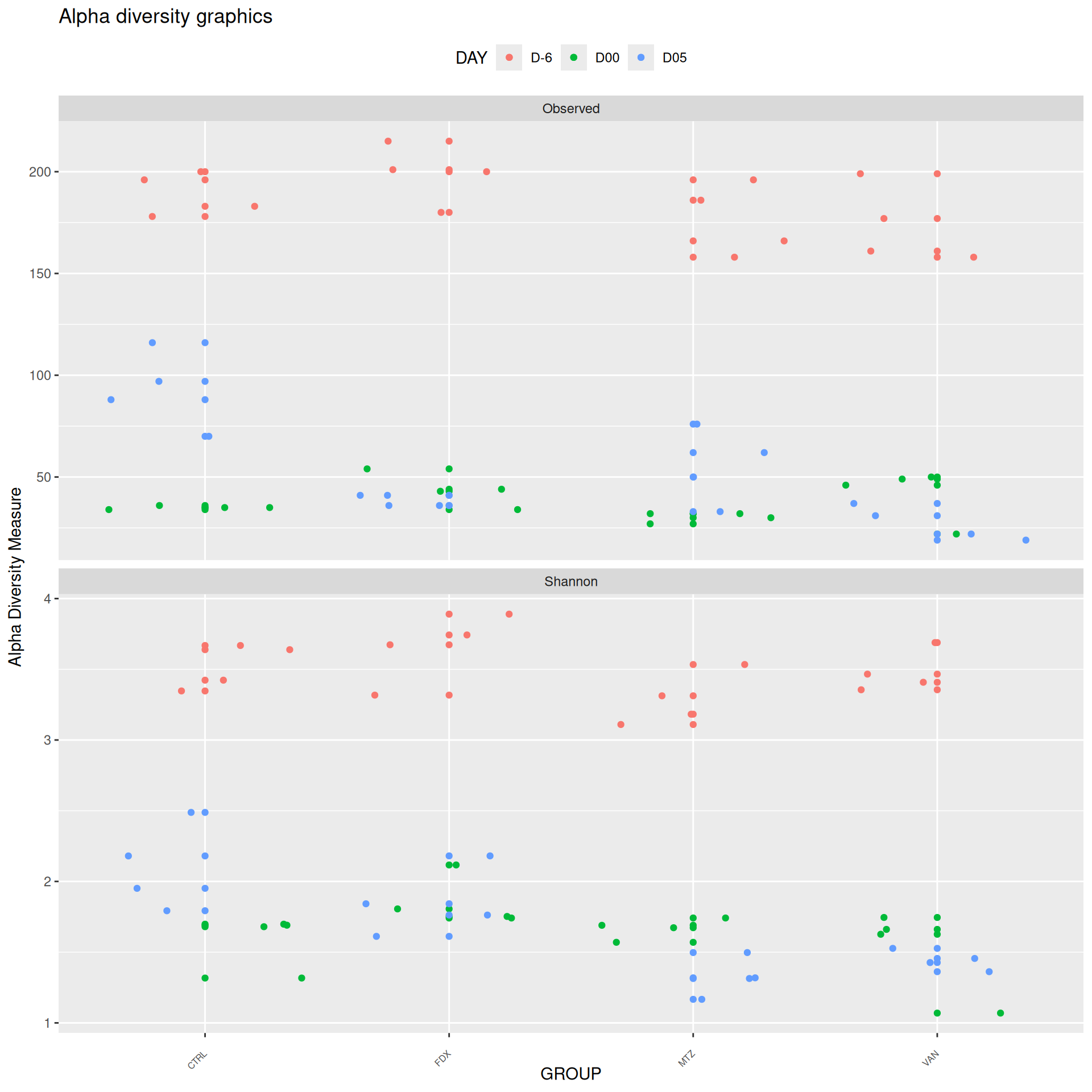
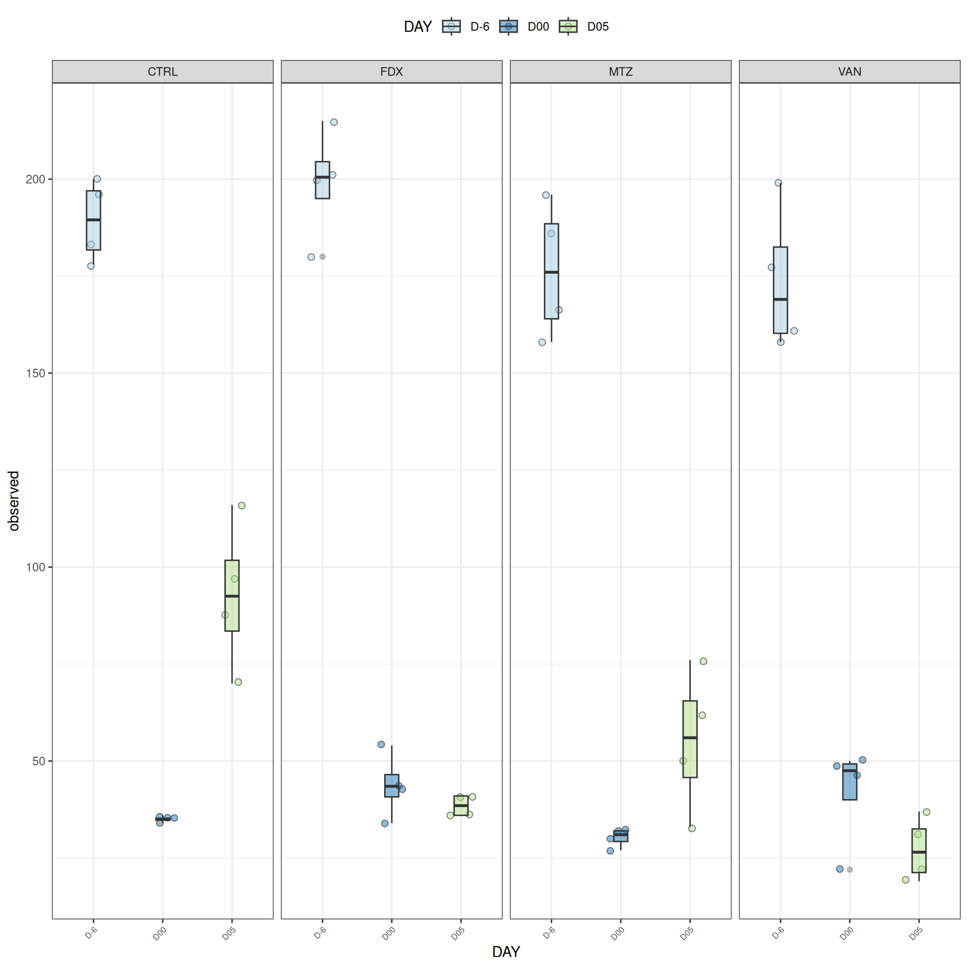
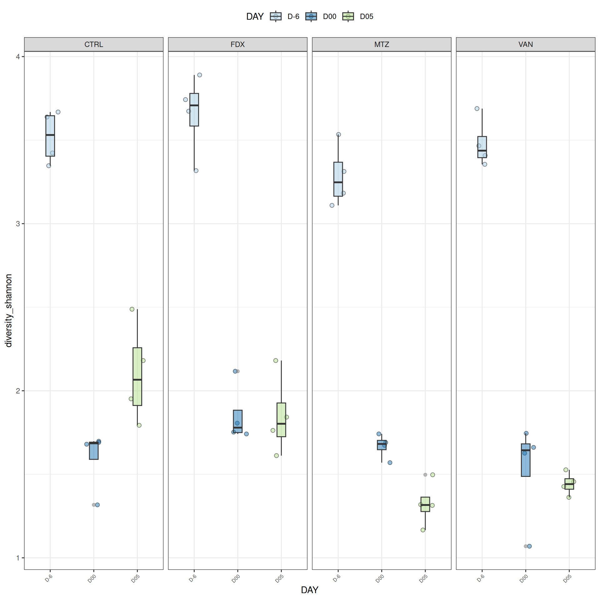
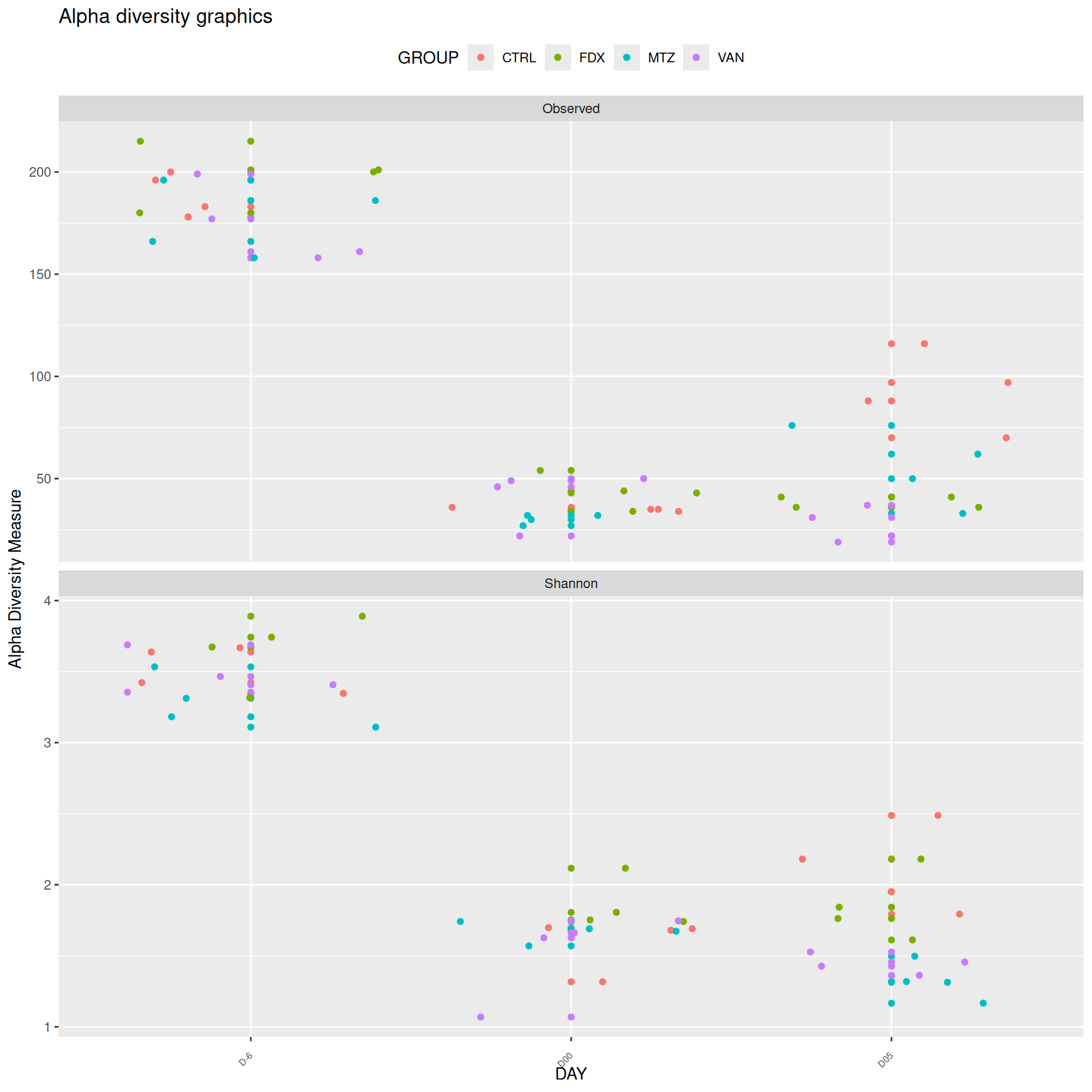
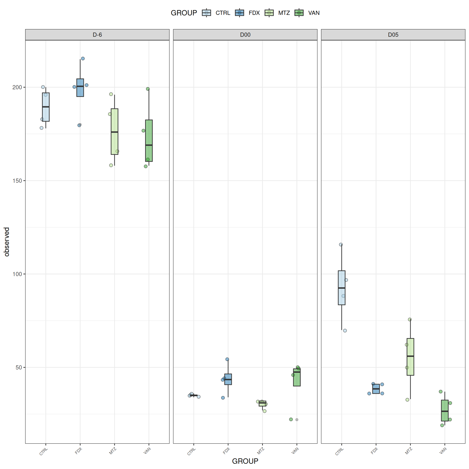
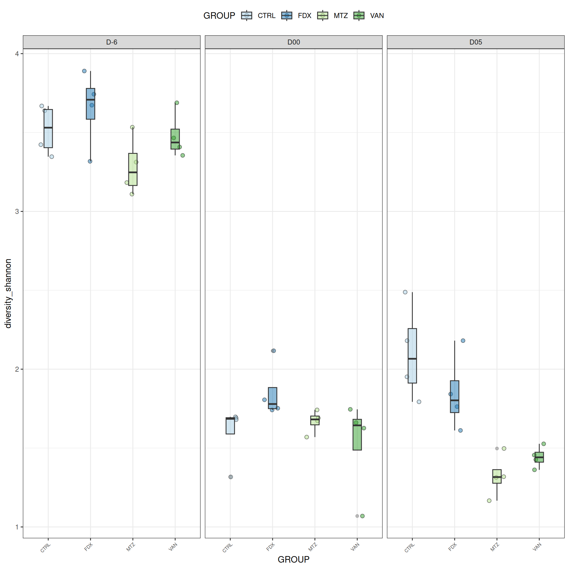
We observed that the alpha-diversity is mainly determined by DAY rather than GROUP. For each sample, the observed index measures the richness in the sample i.e. the total number of species in the community. Richness was highest in samples from J-6 and J51, and also J28 with more variability. It decreased on J00, and J37 on days of infection, and increased between infection dates. The other indices do not provide any additional information, as the trajectories are consistent with infection dates.
Alpha-diversity - statistical tests
We calculated the alpha-diversity indices and combined them with covariates from experimental design.
#model <- aov(Observed ~ DAY*GROUP, data = div_data)#anova(model)#coef(model)# produce parwise comparison test with Tukey's post-hoc correction #TukeyHSD(model, which ="DAY:GROUP")alphadiv.lm <-lm(Observed ~ DAY*GROUP, data = div_data)anova(alphadiv.lm)
Analysis of Variance Table

Response: Observed
          Df Sum Sq Mean Sq  F value    Pr(>F)
DAY        6 321240   53540 241.2943 < 2.2e-16 ***
GROUP      3  11936    3979  17.9318 4.398e-09 ***
DAY:GROUP 18  25966    1443   6.5013 9.870e-10 ***
Residuals 84  18638     222
---
Signif. codes:  0 '***' 0.001 '**' 0.01 '*' 0.05 '.' 0.1 ' ' 1
Show the code
# interaction visualisationpar(mfrow =c(1,2))emmip(alphadiv.lm, GROUP ~ DAY, CIs =TRUE)
Show the code
emmip(alphadiv.lm, DAY ~ GROUP, CIs =TRUE)
Show the code
par(mfrow =c(1,1))#tests EMM <-emmeans(alphadiv.lm, ~ DAY*GROUP)# tests correction are performed within the variable# P value adjustment: tukey method for comparing a family of 12 estimatescomp1 <-pairs(EMM, simple ="DAY")# P value adjustment: tukey method for comparing a family of 5 estimates comp2 <-pairs(EMM, simple ="GROUP")
Show the code
# P value adjustment: tukey method for comparing a family of 60 estimates res_emm <-contrast(EMM, method ="revpairwise", by =NULL, enhance.levels =c("DAY", "GROUP"), adjust ="tukey")
Important
Richness is significantly different by DAY, GROUP and also by the interaction DAY:GROUP. Pairwise tests between DAY, GROUP and also by the interaction DAY:GROUPwere performed with post hoc Tukey’s test to determine which were significant.
Beta-diversity excluding R treatment
The dissimilarity between samples based on taxonomic composition is calculated with one of these Beta diversities: Bray-Curtis, Unweighted and weighted Unifrac, Jaccard index. The Jaccard index uses presence/absence information only whereas UniFrac integrates information from the phylogenetic tree.
Show the code
# use all samples from the complete study frogs_raredist.jac <- phyloseq::distance(frogs_rare, method ="cc")dist.bc <- phyloseq::distance(frogs_rare, method ="bray")dist.uf <- phyloseq::distance(frogs_rare, method ="unifrac")dist.wuf <- phyloseq::distance(frogs_rare, method ="wunifrac")distance_list <-list("Jaccard"= dist.jac,"Bray-Curtis"= dist.bc# "UniFrac" = dist.uf,# "wUniFrac" = dist.wuf)
# Mahendra's function# used own color's palette and shapemy_pcoa_with_arrows2 <-function(physeq = mydata_rare, variable1, variable2, shapeval, colorpal) {# select samples of interest where all samples were used to calculate the distances between samples # dist.jac is previously calculated with all samples of the study#dist.c <- phyloseq::distance(physeq, "jaccard") dist.c <- dist.jac %>%as.matrix() %>%`[`(sample_names(physeq), sample_names(physeq)) %>%as.dist() ord.c <-ordinate(physeq, "MDS", dist.c) p <-plot_ordination(physeq, ord.c)# ## Build arrow data plot_data <- p$data arrow_data <- plot_data %>%group_by(pick({{variable2}}, {{variable1}})) %>%arrange({{variable1}}) %>%mutate(xend = Axis.1, xstart =lag(xend),yend = Axis.2, ystart =lag(yend) )## Plot with arrows p +aes(shape = .data[[ variable2 ]], color = .data[[ variable1 ]]) +scale_shape_manual(values = shapeval) +scale_color_manual(name = colorpal$name,labels = colorpal$labels,values = colorpal$values) +theme_bw() +geom_segment(data = arrow_data,aes(x = xstart, y = ystart, xend = xend, yend = yend),size =0.8, linetype ="3131",arrow =arrow(length=unit(0.1,"inches")),show.legend =FALSE) +geom_point(size =3) +theme(legend.position ="bottom")}
Show the code
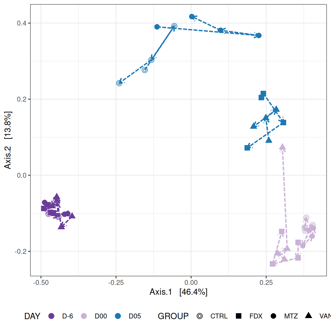
# MDS plot for samples of interests # from distance calculated with all samples of the complete study# used https://colorbrewer2.org/#type=qualitative&scheme=Paired&n=12Jour_pal <-list(name ="DAY",labels =c("D-6", "D00", "D02", "D05", "D07", "D14", "D28"),values =c("#6a3d9a", "#cab2d6", "#a6cee3", "#1f78b4", "#33a02c", "#b2df8a", "#fdbf6f"))GROUP_shape <-list(values =c(1, 15, 16, 17))my_plot2(variable1 ="DAY",variable2 ="GROUP",physeq = frogs_rare_withoutR,shapeval = GROUP_shape$values,colorpal = Jour_pal )
We use the Jaccard distance and show MDS trajectories of the communities intra conditions.
Show the code
# MDS plot for samples of interests # from distance calculated with all samples of the complete study# used https://colorbrewer2.org/#type=qualitative&scheme=Paired&n=12p <-my_pcoa_with_arrows2(variable1 ="DAY",variable2 ="GROUP",physeq = frogs_rare_withoutR,shapeval = GROUP_shape$values,colorpal = Jour_pal)p
Important
The Multidimensional scaling (MDS / PCoA) showed that samples were distributed according to the variable DAY on the first two axes. Samples from J-6, J28 and J51 are homogeneous, close to each other and opposite to samples from J00 on the first axis. The others are distributed in both dimensions.
Permutation test for adonis under reduced model
Permutation: free
Number of permutations: 9999

vegan::adonis2(formula = dist.bc ~ DAY * GROUP, data = metadata, permutations = 9999)
          Df SumOfSqs      R2      F Pr(>F)
Model     27   26.762 0.82047 14.218  1e-04 ***
Residual  84    5.856 0.17953
Total    111   32.618 1.00000
---
Signif. codes:  0 '***' 0.001 '**' 0.01 '*' 0.05 '.' 0.1 ' ' 1
Important
The change in microbiota composition measured by the Bray-Curtis Beta diversity is significantly different between DAY, GROUP and also between the levels of the interaction factor DAY:GROUP at 0.05 significance level. The influence of the factors differs between ecosystems.
Annex3: study on subset dysbiose excluding R treatment
Important
Note that the rarefaction was performed on all samples from the complete study. We extracted samples of interest from the frogs_rare phyloseq object to calculate alpha diversity. Alpha diversity is calculated within sample and do not change with the previous analyses on the complete study.
Show the code
frogs_rare_dysbiose_withoutR <-subset_samples(frogs_rare, DAY %in%c("D-6", "D00", "D05") & GROUP !="R")
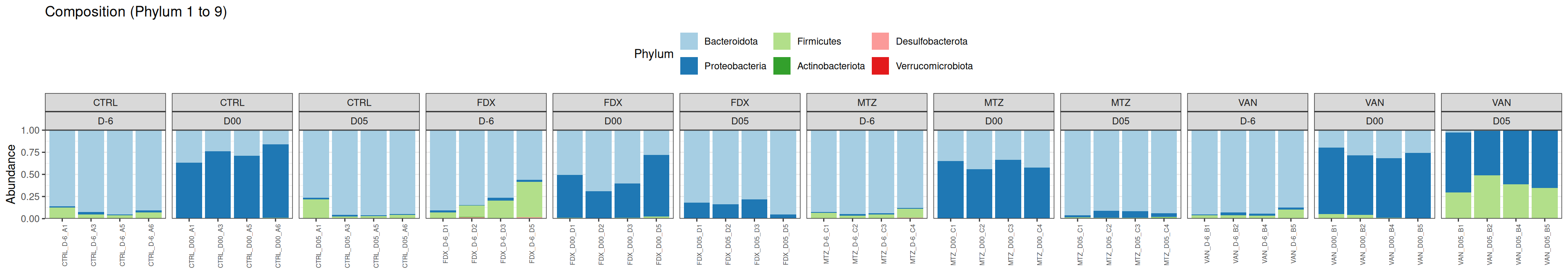
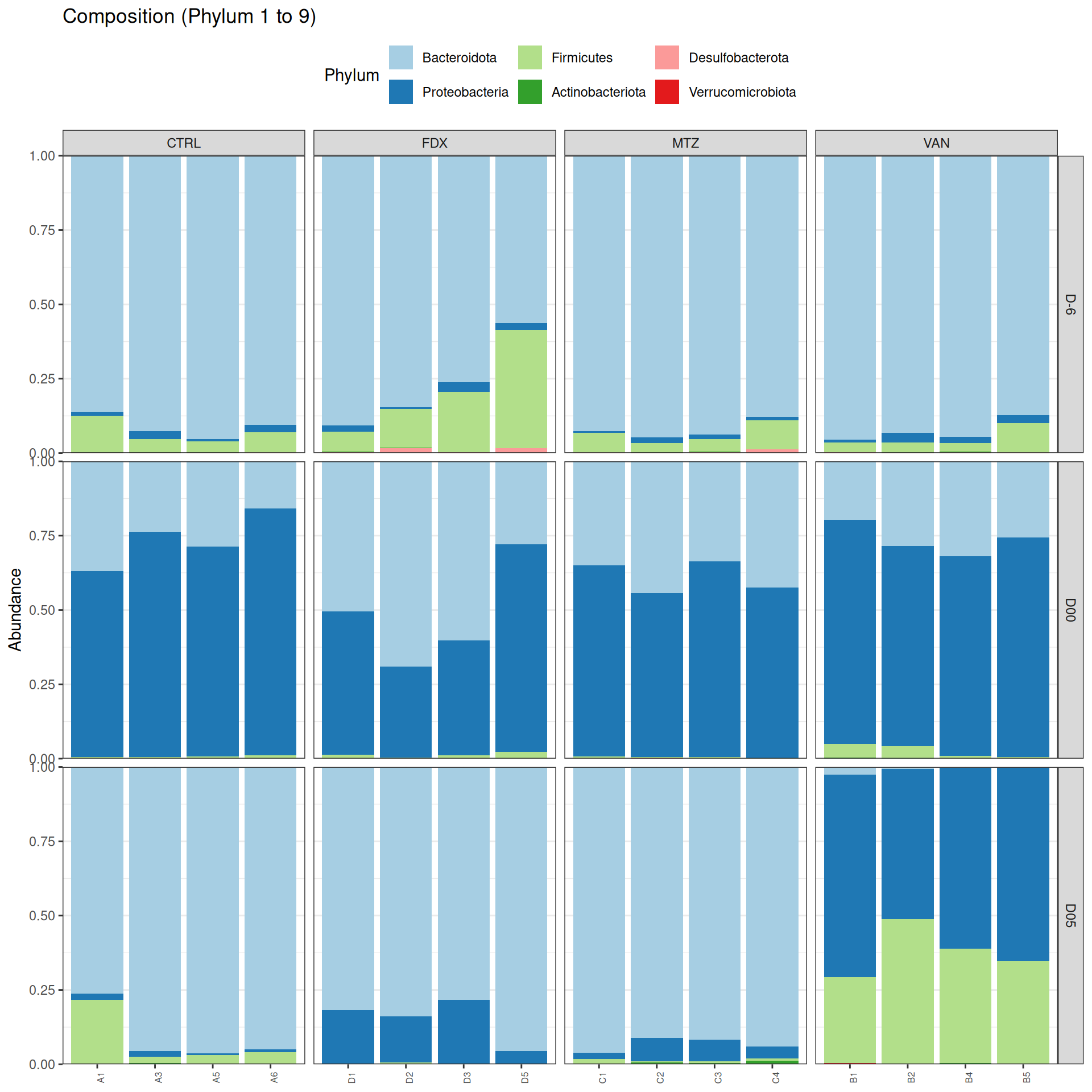
Taxonomic composition
After rarefaction, let’s have a look at the Phylum and genus levels composition with two types of plot.
Problematic taxa
                 taxa  Kingdom     Phylum      Class                      Order
Cluster_27 Cluster_27 Bacteria Firmicutes Clostridia Clostridia vadinBB60 group
            Family rank
Cluster_27 Unknown    8
Alpha-Diversity on subset dysbiose excluding R treatment
#model <- aov(Observed ~ DAY*GROUP, data = div_data)#anova(model)#coef(model)# produce parwise comparison test with Tukey's post-hoc correction #TukeyHSD(model, which ="DAY:GROUP")alphadiv.lm <-lm(Observed ~ DAY*GROUP, data = div_data)anova(alphadiv.lm)
Analysis of Variance Table

Response: Observed
          Df Sum Sq Mean Sq  F value    Pr(>F)
DAY        2 208261  104130 624.1575 < 2.2e-16 ***
GROUP      3   4013    1338   8.0183 0.0003207 ***
DAY:GROUP  6   7930    1322   7.9220 1.752e-05 ***
Residuals 36   6006     167
---
Signif. codes:  0 '***' 0.001 '**' 0.01 '*' 0.05 '.' 0.1 ' ' 1
Show the code
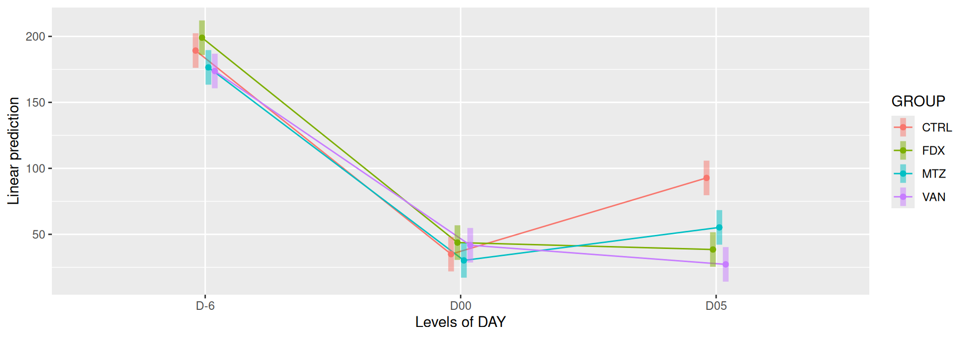
# interaction visualisationpar(mfrow =c(1,2))emmip(alphadiv.lm, GROUP ~ DAY, CIs =TRUE)
Show the code
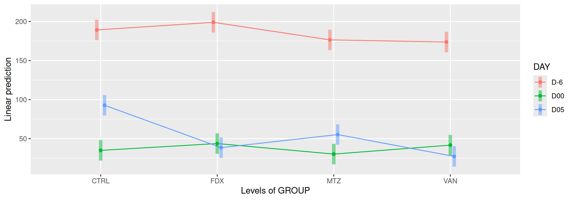
emmip(alphadiv.lm, DAY ~ GROUP, CIs =TRUE)
Show the code
par(mfrow =c(1,1))#tests EMM <-emmeans(alphadiv.lm, ~ DAY*GROUP)# tests correction are performed within the variable# P value adjustment: tukey method for comparing a family of 12 estimatescomp1 <-pairs(EMM, simple ="DAY")# P value adjustment: tukey method for comparing a family of 5 estimates comp2 <-pairs(EMM, simple ="GROUP")
Show the code
# P value adjustment: tukey method for comparing a family of 60 estimates res_emm <-contrast(EMM, method ="revpairwise", by =NULL, enhance.levels =c("DAY", "GROUP"), adjust ="tukey")
Important
Richness is significantly different by DAY, GROUP and also by the interaction DAY:GROUP. Pairwise tests between DAY, GROUP and also by the interaction DAY:GROUPwere performed with post hoc Tukey’s test to determine which were significant.
Beta-diversity on subset dysbiose excluding R treatment
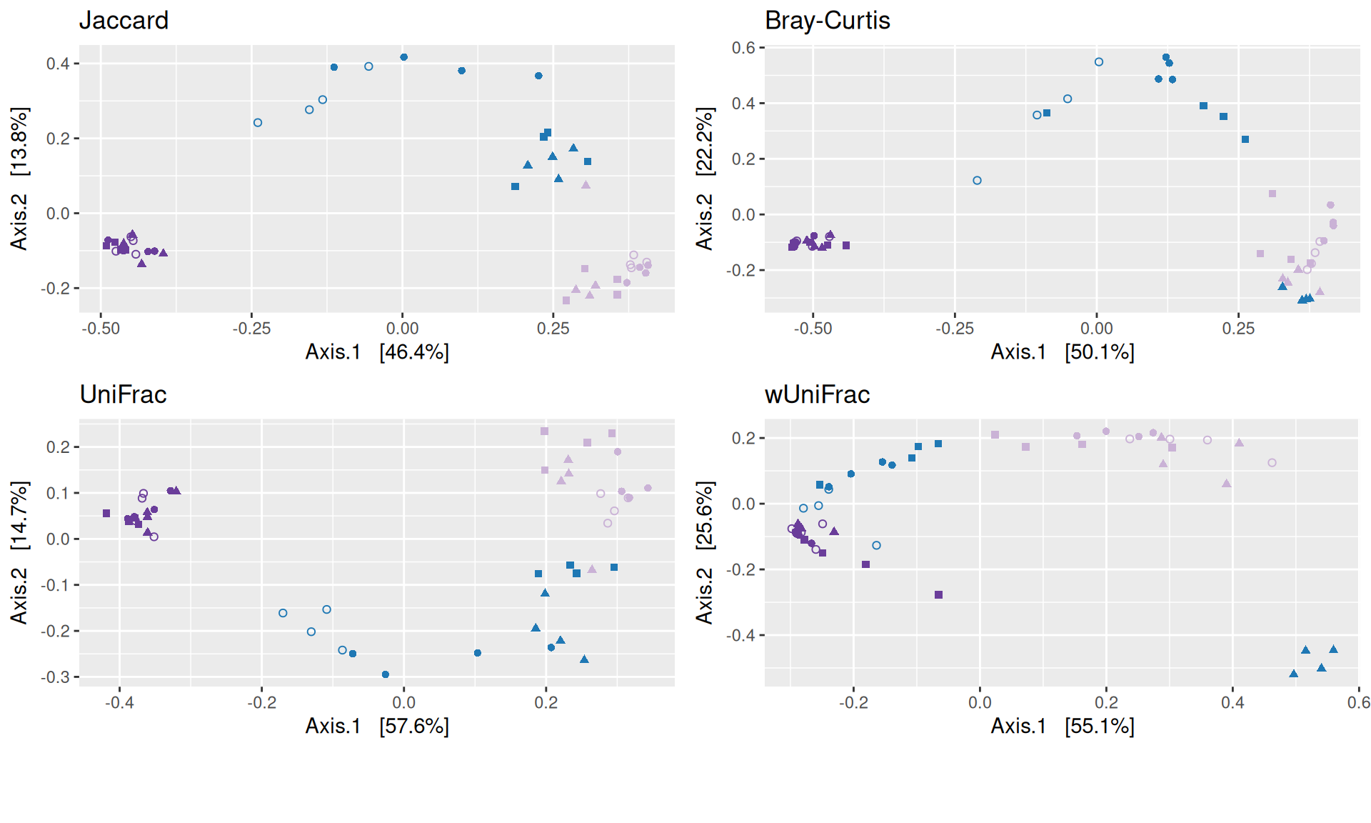
The dissimilarity between samples based on taxonomic composition is calculated with one of these Beta diversities: Bray-Curtis, Unweighted and weighted Unifrac, Jaccard index. The Jaccard index uses presence/absence information only whereas UniFrac integrates information from the phylogenetic tree.
Show the code
# use all samples from the complete study frogs_raredist.jac <- phyloseq::distance(frogs_rare, method ="cc")dist.bc <- phyloseq::distance(frogs_rare, method ="bray")dist.uf <- phyloseq::distance(frogs_rare, method ="unifrac")dist.wuf <- phyloseq::distance(frogs_rare, method ="wunifrac")distance_list <-list("Jaccard"= dist.jac,"Bray-Curtis"= dist.bc,"UniFrac"= dist.uf,"wUniFrac"= dist.wuf)
# Mahendra's function# used own color's palette and shapemy_pcoa_with_arrows2 <-function(physeq = mydata_rare, variable1, variable2, shapeval, colorpal) {# select samples of interest where all samples were used to calculate the distances between samples # dist.jac is previously calculated with all samples of the study#dist.c <- phyloseq::distance(physeq, "jaccard") dist.c <- dist.jac %>%as.matrix() %>%`[`(sample_names(physeq), sample_names(physeq)) %>%as.dist() ord.c <-ordinate(physeq, "MDS", dist.c) p <-plot_ordination(physeq, ord.c)# ## Build arrow data plot_data <- p$data arrow_data <- plot_data %>%group_by(pick({{variable2}}, {{variable1}})) %>%arrange({{variable1}}) %>%mutate(xend = Axis.1, xstart =lag(xend),yend = Axis.2, ystart =lag(yend) )## Plot with arrows p +aes(shape = .data[[ variable2 ]], color = .data[[ variable1 ]]) +scale_shape_manual(values = shapeval) +scale_color_manual(name = colorpal$name,labels = colorpal$labels,values = colorpal$values) +theme_bw() +geom_segment(data = arrow_data,aes(x = xstart, y = ystart, xend = xend, yend = yend),size =0.8, linetype ="3131",arrow =arrow(length=unit(0.1,"inches")),show.legend =FALSE) +geom_point(size =3) +theme(legend.position ="bottom")}
Show the code
# MDS plot for samples of interests # from distance calculated with all samples of the complete study# used https://colorbrewer2.org/#type=qualitative&scheme=Paired&n=12Jour_pal <-list(name ="DAY",labels =c("D-6", "D00", "D05"),values =c("#6a3d9a", "#cab2d6", "#1f78b4"))GROUP_shape <-list(values =c(1, 15, 16, 17))my_plot2(variable1 ="DAY",variable2 ="GROUP",physeq = frogs_rare_dysbiose_withoutR,shapeval = GROUP_shape$values,colorpal = Jour_pal )
We use the Jaccard distance and show MDS trajectories of the communities intra conditions.
Show the code
# MDS plot for samples of interests # from distance calculated with all samples of the complete study# used https://colorbrewer2.org/#type=qualitative&scheme=Paired&n=12p <-my_pcoa_with_arrows2(variable1 ="DAY",variable2 ="GROUP",physeq = frogs_rare_dysbiose_withoutR,shapeval = GROUP_shape$values,colorpal = Jour_pal)p
Important
The Multidimensional scaling (MDS / PCoA) showed that samples were distributed according to the variable DAY on the first two axes. Samples from J-6, J28 and J51 are homogeneous, close to each other and opposite to samples from J00 on the first axis. The others are distributed in both dimensions.
Permutation test for adonis under reduced model
Permutation: free
Number of permutations: 9999

vegan::adonis2(formula = dist.bc ~ DAY * GROUP, data = metadata, permutations = 9999)
         Df SumOfSqs     R2      F Pr(>F)
Model    11  11.5949 0.8223 15.144  1e-04 ***
Residual 36   2.5057 0.1777
Total    47  14.1006 1.0000
---
Signif. codes:  0 '***' 0.001 '**' 0.01 '*' 0.05 '.' 0.1 ' ' 1
Important
The change in microbiota composition measured by the Bray-Curtis Beta diversity is significantly different between DAY, GROUP and also between the levels of the interaction factor DAY:GROUP at 0.05 significance level. The influence of the factors differs between ecosystems.
1. McMurdie PJ, Holmes S. Phyloseq: An r package for reproducible interactive analysis and graphics of microbiome census data. PloS one. 2013;8:e61217.
This document will not be accessible without prior agreement of the partners
A work by Migale Bioinformatics Facility
Université Paris-Saclay, INRAE, MaIAGE, 78350, Jouy-en-Josas, France
Université Paris-Saclay, INRAE, BioinfOmics, MIGALE bioinformatics facility, 78350, Jouy-en-Josas, France
Source Code
---title: "ICD"search: falsenavbar: falsesubtitle: "Accompaniement of Anaïs Brosse in her analyses"author: - name: Olivier Rué orcid: 0000-0003-1689-0557 email: olivier.rue@inrae.fr affiliations: - name: Migale bioinformatics facility adress: Domaine de Vilvert city: Jouy-en-Josas state: France - name: Christelle Hennequet-Antier orcid: 0000-0001-5836-2803 email: christelle.hennequet-antier@inrae.fr affiliations: - name: Migale bioinformatics facility adress: Domaine de Vilvert city: Jouy-en-Josas state: Francedate: "2023-07-05"date-modified: todayimage: "images/preview.jpg"reader-mode: falsefig-cap-location: bottomtbl-cap-location: toplicense: "This document will not be accessible without prior agreement of the partners"format: html: embed-resources: false toc: true code-fold: true code-summary: "Show the code" code-tools: true toc-location: right page-layout: article code-overflow: wrap---```{r setup, include=FALSE}knitr::opts_chunk$set(eval=TRUE, echo =TRUE, cache = FALSE, message = FALSE, warning = FALSE, cache.lazy = FALSE, fig.height = 3.5, fig.width = 10)``````{r}#| label: load-packages#library(DT)library(tidyverse)#library(kableExtra)library(phyloseq)library(phyloseq.extended)library(data.table)library(InraeThemes)library(readr) #read_delimlibrary(ggplot2) # graphicslibrary(microbiome) # for boxplot_alpha functionlibrary(mia) # microbiome analysis with SummarizedExperiment and TreeSummarizedExperimentlibrary(microViz) # analysis and visualization of microbiome sequencing datalibrary(emmeans) #post hoc testslibrary(reactable) #table formatting and stylinglibrary(reactablefmtr) #table formatting and stylinglibrary(openxlsx) #save results to excel sheetslibrary(ggtree) # visualizationlibrary(ggtreeExtra) # visualizationlibrary(stringr) # manipulate string```<!-- ```{r datatable global options, echo=FALSE, eval=TRUE} --><!-- options(DT.options = list(pageLength = 10, --><!-- scrollX = TRUE, --><!-- language = list(search = 'Filter:'), --><!-- dom = 'lftipB', --><!-- buttons = c('copy', 'csv', 'excel'))) --><!-- ``` -->{{< include /resources/_includes/_intro_note.qmd >}}# Aim of the projectInfluence of treatment antibiotics in a murine model of infection with *Clostridium difficile* (ICD). Injection of *C. difficile* were performed at `J00` and `J37`.- Différencier les groupes ctrl et traités aux antibiotiques (VAN, MTZ, FDX, R = réinfections multiples), et comparer les cinétiques entre les groupes.- Etudier les cinétiques au sein des traitements (CTRL, VAN, MTZ, FDX, R). Est-ce qu’il y a un retour à J-6 ? Clairance de la bactérie (zéro dans les fécès, attention biofilm et sporulation peuvent encore existés)- Eubiose : comparer J-6, J28, J51. ## Partners* Olivier Rué - Migale bioinformatics facility - BioInfomics - INRAE* Christelle Hennequet-Antier - Migale bioinformatics facility - BioInfomics - INRAE* Mahendra Mariadassou - Migale bioinformatics facility - BioInfomics - INRAE* Anaïs Brosse - MICALIS - INRAE# Data management{{< include /resources/_includes/_data_management.qmd >}}# Analyses## Experiment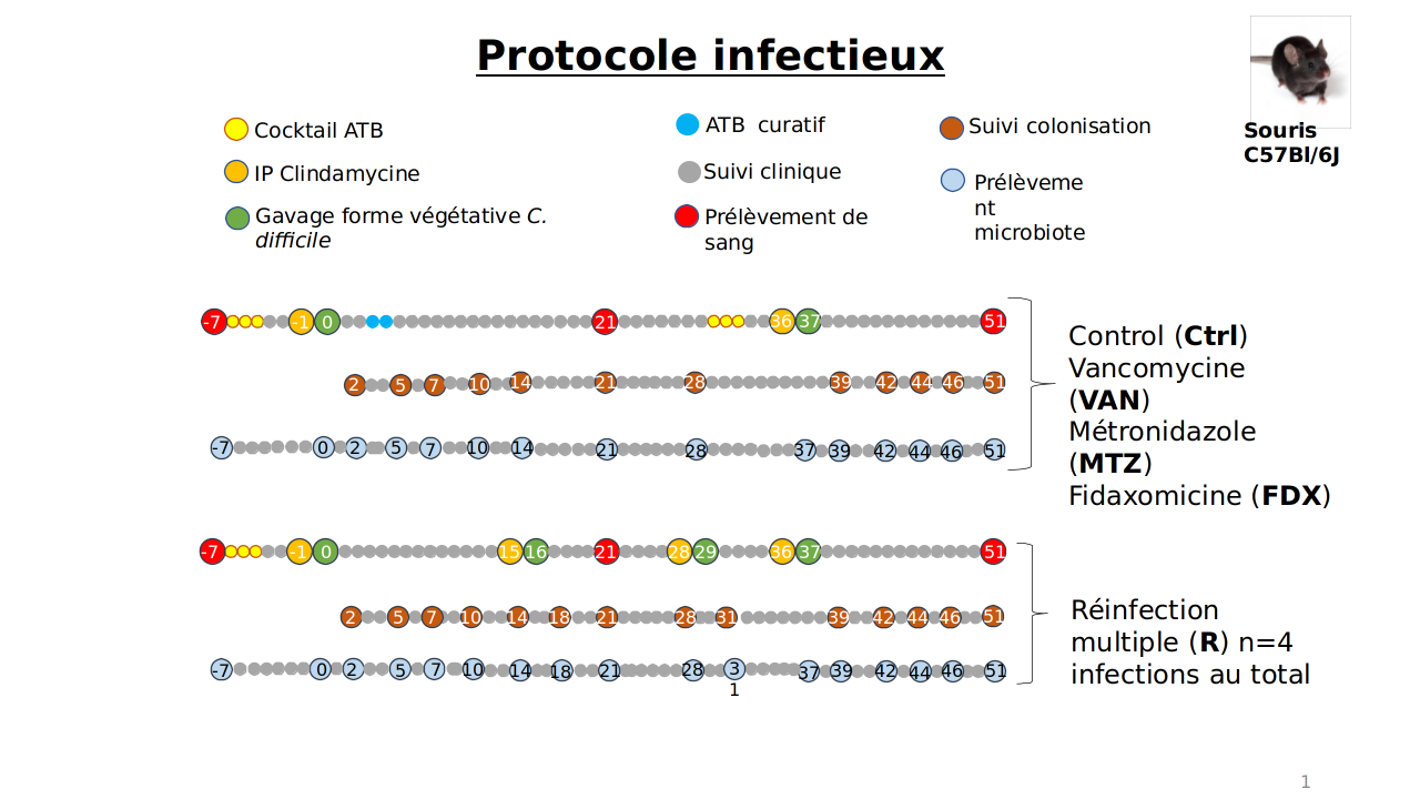{fig-align="center"}## Phyloseq object creation{{< include /resources/_includes/_phyloseq.qmd >}}```{r}#| label: phyloseqOjectbiomfile <-"../data/Galaxy17-[FROGS_Affiliation_OTU__affiliation_abundance.biom].biom1"frogs <-import_frogs(biomfile, taxMethod ="blast",treefilename ="../data/Galaxy20-[FROGS_Tree__tree.nwk].nhx")metadata_allsamples <-read_delim("../data/metadata-allsamples.csv", delim =";", escape_double =FALSE, col_types =cols(SAMPLE_ID =col_character(), GROUPE = vroom::col_factor(levels =c("CTRL", "FDX", "MTZ", "VAN", "R")), REPLICAT = vroom::col_factor(levels =c("1", "2", "3", "4")),JOUR = vroom::col_factor(levels =c("J-6", "J0", "J2", "J5", "J7", "J14", "J18", "J28", "J31", "J37", "J39", "J51"))),trim_ws =TRUE) %>%column_to_rownames(var="SAMPLE_ID")#rename variables into englishmetadata_allsamples <- dplyr::rename(metadata_allsamples, DAY = JOUR)metadata_allsamples <- dplyr::rename(metadata_allsamples, GROUP = GROUPE)#put new label for the JOUR levels to be ordered#metadata_allsamples$JOUR <- factor(metadata_allsamples$JOUR, levels = c("J-6", "J0", "J2", "J5", "J7", "J14", "J18", "J28", "J31", "J37", "J39", "J51"), labels = c("J-6", "J00", "J02", "J05", "J07", "J14", "J18", "J28", "J31", "J37", "J39", "J51"))metadata_allsamples$DAY <-factor(metadata_allsamples$DAY, levels =c("J-6", "J0", "J2", "J5", "J7", "J14", "J18", "J28", "J31", "J37", "J39", "J51"), labels =c("D-6", "D00", "D02", "D05", "D07", "D14", "D18", "D28", "D31", "D37", "D39", "D51"))# EUBIOSE <- J-6# EUBIOSE <- J28# EUBIOSE <- J51# Other maner to include phylogenetic tree# phy_tree(frogs) <- read_tree("../data/Galaxy20-[FROGS_Tree__tree.nwk].nhx")# Explore sample infossample_data(frogs) <- metadata_allsamples# add new variables to facilitate visualisation and statistical testssample_data(frogs) <- metadata_allsamples %>%mutate(Label =paste(GROUP, DAY, SOURIS, sep="_")) %>%mutate(GROUPJ =factor(paste(GROUP, DAY, sep="_")))# change name of samplessample_names(frogs) <-sample_data(frogs) %>%as_tibble() %>% dplyr::select(Label) %>%t()# sample_data(frogs)# info phyloseq object#reorder samplesfrogs <- frogs %>% microViz::ps_arrange(DAY, GROUP)frogsmicrobiome::summarize_phyloseq(frogs)# save phyloseq object#saveRDS(object = frogs, file="./html/frogs.rds")saveRDS(object = frogs, file="./frogs.rds")``````{r}#| label: checkdesign# count number of replicate by # - GROUP# - combination of GROUP and DAYsample_data(frogs) %>%as_tibble() %>% dplyr::count(GROUP) sample_data(frogs) %>%as_tibble() %>% dplyr::add_count(GROUP, DAY) %>% dplyr::select(GROUP, DAY, GROUPJ, n) %>%distinct() %>%ggplot(., aes(x = GROUPJ, y = n, fill = GROUP)) +geom_bar(stat ="identity") +labs(title="Number of replicates", y ="n") +theme(axis.title.x =element_blank(),axis.text.x =element_text(angle =90, size =8, hjust =1))# frequencies within each DAY for the levels of GROUPmicrobiome::plot_frequencies(sample_data(frogs), "DAY", "GROUP")```<!-- ## Taxonomic composition with rawdata --><!-- ```{r} --><!-- #| label: compos_rawdata_init --><!-- phyloseq.extended::plot_composition(physeq = frogs, taxaRank1 = "Kingdom", taxaSet1 = "Bacteria", taxaRank2 = "Phylum", numberOfTaxa = 10L) + --><!-- facet_grid(~GROUP, scales = "free_x", space = "free") + --><!-- theme(axis.text.x = element_text(size = 6, hjust = 1)) + --><!-- theme(legend.position="top") --><!-- ``` --><!-- ```{r} --><!-- phyloseq.extended::plot_composition(physeq = frogs, taxaRank1 = "Kingdom", taxaSet1 = "Bacteria", taxaRank2 = "Genus", numberOfTaxa = 10L) + --><!-- facet_grid(~GROUP, scales = "free_x", space = "free") + --><!-- theme(axis.text.x = element_text(size = 6, hjust = 1)) + --><!-- theme(legend.position="top") --><!-- ``` --><!-- ```{r} --><!-- #subsetting with GROUP value --><!-- phyloseq.extended::plot_composition(physeq = subset_samples(frogs, GROUP == "CTRL"), taxaRank1 = "Kingdom", taxaSet1 = "Bacteria", taxaRank2 = "Phylum", numberOfTaxa = 10L) + --><!-- facet_grid(~DAY, scales = "free_x", space = "free") + --><!-- theme(axis.text.x = element_text(size = 8, hjust = 1)) + --><!-- theme(legend.position="top") --><!-- ``` -->## RarefactionSamples from `J-6` provided less abundances than the others.```{r}#| label: plot_barphyloseq::plot_bar(frogs, fill="Phylum")```For having the same sampling depth for all samples, we rarefy them before exploring the diversity.```{r}#| label: frogs_rarefrogs_rare <- phyloseq::rarefy_even_depth(frogs, rngseed =123, replace =TRUE)```All depths are now equal to `r as.integer(min(phyloseq::sample_sums(frogs)))`. The dataset contains `r as.integer(sum(phyloseq::sample_sums(frogs_rare)))` sequences allocated to `r as.integer(phyloseq::ntaxa(frogs_rare))` taxa. Bacteroidota and Proteobateria are dominants. ```{r}#| label: plot_bar_rarephyloseq::plot_bar(frogs_rare, x="REPLICAT", fill="Phylum") +facet_grid(GROUP~DAY, scales="free_x")```## Taxonomic compositionThe taxonomic composition is studied after rarefaction. Let's have a look at the Phylum level composition. Fermicutes are also present up to 50% depending on the `GROUP` and the `DAY` variables. They disappear at J00, J02 J37, except J37 with `R` treatment.::: {.panel-tabset}### After rarefaction```{r}#| label: compos_rarephyloseq.extended::plot_composition(physeq = frogs_rare, taxaRank1 ="Kingdom", taxaSet1 ="Bacteria", taxaRank2 ="Phylum", numberOfTaxa =10L) +facet_grid(~GROUP, scales ="free_x", space ="free") +scale_fill_brewer(palette ="Paired") +theme(axis.text.x =element_text(size =6, hjust =1)) +theme(legend.position="top")```### Before rarefaction```{r}#| label: compos_rawdataphyloseq.extended::plot_composition(physeq = frogs, taxaRank1 ="Kingdom", taxaSet1 ="Bacteria", taxaRank2 ="Phylum", numberOfTaxa =10L) +facet_grid(~GROUP, scales ="free_x", space ="free") +scale_fill_brewer(palette ="Paired") +theme(axis.text.x =element_text(size =6, hjust =1)) +theme(legend.position="top")```:::After rarefaction, let's have a look at the Phylum and genus levels composition with two types of plot.We explore composition using all samples.::: {.panel-tabset}### All By GROUP```{r}#| label: All_compos_rare_by_GROUP#| fig-width: 20#| class: superbigimagephyloseq.extended::plot_composition(frogs_rare, NULL, NULL, "Phylum") +facet_grid(~ GROUP + DAY, scales ="free_x", space ="free_x") +scale_fill_brewer(palette ="Paired") +theme(axis.text.x =element_text(size =6, hjust =1)) +theme(legend.position="top")```### All By grid at phylum level```{r}#| label: All_compos_rare_by_GROUP_DAY#| fig-height: 10phyloseq.extended::plot_composition(frogs_rare, NULL, NULL, "Phylum", x ="SOURIS") +facet_grid(rows =vars(DAY), cols =vars(GROUP), scales ="free_x", space ="free_x") +scale_fill_brewer(palette ="Paired") +theme(axis.text.x =element_text(size =6, hjust =1)) +theme(legend.position="top")```### All By grid at family level```{r}#| label: All_compos_rare_by_GROUP_DAY_family#| fig-height: 10phyloseq.extended::plot_composition(frogs_rare, NULL, NULL, "Family", x ="SOURIS") +facet_grid(rows =vars(DAY), cols =vars(GROUP), scales ="free_x", space ="free_x") +scale_fill_brewer(palette ="Paired") +theme(axis.text.x =element_text(size =6, hjust =1)) +theme(legend.position="top")```### All By grid at genus level```{r}#| label: All_compos_rare_by_GROUP_DAY_genus#| fig-height: 10phyloseq.extended::plot_composition(frogs_rare, NULL, NULL, "Genus", x ="SOURIS") +facet_grid(rows =vars(DAY), cols =vars(GROUP), scales ="free_x", space ="free_x") +scale_fill_brewer(palette ="Paired") +theme(axis.text.x =element_text(size =6, hjust =1)) +theme(legend.position="top")```:::To explore presence of bacteria at genus levels within phylum:::: {.panel-tabset}### Bacteroidota```{r}#| label: All_compos_rare_Bacteroidota#| fig-height: 10phyloseq.extended::plot_composition(frogs_rare, "Phylum", "Bacteroidota", "Genus", fill ="Genus", x ="SOURIS") +facet_grid(rows =vars(DAY), cols =vars(GROUP), scales ="free_x", space ="free_x") +scale_fill_brewer(palette ="Paired") +theme(axis.text.x =element_text(size =6, hjust =1)) +theme(legend.position="top")```### Proteobacteria```{r}#| label: All_compos_rare_Proteobacteria#| fig-height: 10phyloseq.extended::plot_composition(frogs_rare, "Phylum", "Proteobacteria", "Genus", fill ="Genus", x ="SOURIS") +facet_grid(rows =vars(DAY), cols =vars(GROUP), scales ="free_x", space ="free_x") +scale_fill_brewer(palette ="Paired") +theme(axis.text.x =element_text(size =6, hjust =1)) +theme(legend.position="top")```### Firmicutes```{r}#| label: All_compos_rare_Firmicutes#| fig-height: 10phyloseq.extended::plot_composition(frogs_rare, "Phylum", "Firmicutes", "Genus", fill ="Genus", x ="SOURIS") +facet_grid(rows =vars(DAY), cols =vars(GROUP), scales ="free_x", space ="free_x") +scale_fill_brewer(palette ="Paired") +theme(axis.text.x =element_text(size =6, hjust =1)) +theme(legend.position="top")```### Actinobacteriota```{r}#| label: All_compos_rare_Actinobacteriota#| fig-height: 10phyloseq.extended::plot_composition(frogs_rare, "Phylum", "Actinobacteriota", "Genus", fill ="Genus", x ="SOURIS") +facet_grid(rows =vars(DAY), cols =vars(GROUP), scales ="free_x", space ="free_x") +scale_fill_brewer(palette ="Paired") +theme(axis.text.x =element_text(size =6, hjust =1)) +theme(legend.position="top")```### Verrucomicrobiota```{r}#| label: All_compos_rare_Verrucomicrobiota#| fig-height: 10phyloseq.extended::plot_composition(frogs_rare, "Phylum", "Verrucomicrobiota", "Genus", fill ="Genus", x ="SOURIS") +facet_grid(rows =vars(DAY), cols =vars(GROUP), scales ="free_x", space ="free_x") +scale_fill_brewer(palette ="Paired") +theme(axis.text.x =element_text(size =6, hjust =1)) +theme(legend.position="top")```:::::: {.callout-important}We observed that the taxonomic composition is mainly determined by `DAY` rather than `GROUP`. Protebacteria are dominant in `J00`, `J02`, `J18` (`GROUP R`) and `J37`. Firmicutes are present at `J-6` (a little), `J05` (CTRL and VAN), `J07` (CTRL, VAN, MTZ), `J14`, `J28`, `J39`, `J51`. At the genus level, similar taxonomic patterns were found in `J00` with `J37` and in `J-6` with `J51`.:::We explore composition excluding R treatment.::: {.panel-tabset}### Without R - By GROUP```{r}#| label: WithoutR_compos_rare_by_GROUP#| fig-width: 20#| class: superbigimagephyloseq.extended::plot_composition(physeq =subset_samples(frogs_rare, GROUP !="R"), NULL, NULL, "Phylum") +facet_grid(~ GROUP + DAY, scales ="free_x", space ="free_x") +scale_fill_brewer(palette ="Paired") +theme(axis.text.x =element_text(size =6, hjust =1)) +theme(legend.position="top")```### Without R - By grid at phylum level```{r}#| label: WithoutR_compos_rare_by_GROUP_DAY#| fig-height: 10phyloseq.extended::plot_composition(physeq =subset_samples(frogs_rare, GROUP !="R"), NULL, NULL, "Phylum", x ="SOURIS") +facet_grid(rows =vars(DAY), cols =vars(GROUP), scales ="free_x", space ="free_x") +scale_fill_brewer(palette ="Paired") +theme(axis.text.x =element_text(size =6, hjust =1)) +theme(legend.position="top")```### Without R - By grid at family level```{r}#| label: WithoutR_compos_rare_by_GROUP_DAY_family#| fig-height: 10phyloseq.extended::plot_composition(physeq =subset_samples(frogs_rare, GROUP !="R"), NULL, NULL, "Family", x ="SOURIS") +facet_grid(rows =vars(DAY), cols =vars(GROUP), scales ="free_x", space ="free_x") +scale_fill_brewer(palette ="Paired") +theme(axis.text.x =element_text(size =6, hjust =1)) +theme(legend.position="top")```### Without R - By grid at genus level```{r}#| label: WithoutR_compos_rare_by_GROUP_DAY_genus#| fig-height: 10phyloseq.extended::plot_composition(physeq =subset_samples(frogs_rare, GROUP !="R"), NULL, NULL, "Genus", x ="SOURIS") +facet_grid(rows =vars(DAY), cols =vars(GROUP), scales ="free_x", space ="free_x") +scale_fill_brewer(palette ="Paired") +theme(axis.text.x =element_text(size =6, hjust =1)) +theme(legend.position="top")```:::To explore presence of bacteria at genus levels within phylum:::: {.panel-tabset}### Bacteroidota```{r}#| label: WithoutR_compos_rare_Bacteroidota#| fig-height: 10phyloseq.extended::plot_composition(physeq =subset_samples(frogs_rare, GROUP !="R"), "Phylum", "Bacteroidota", "Genus", fill ="Genus", x ="SOURIS") +facet_grid(rows =vars(DAY), cols =vars(GROUP), scales ="free_x", space ="free_x") +scale_fill_brewer(palette ="Paired") +theme(axis.text.x =element_text(size =6, hjust =1)) +theme(legend.position="top")```### Proteobacteria```{r}#| label: WithoutR_compos_rare_Proteobacteria#| fig-height: 10phyloseq.extended::plot_composition(physeq =subset_samples(frogs_rare, GROUP !="R"), "Phylum", "Proteobacteria", "Genus", fill ="Genus", x ="SOURIS") +facet_grid(rows =vars(DAY), cols =vars(GROUP), scales ="free_x", space ="free_x") +scale_fill_brewer(palette ="Paired") +theme(axis.text.x =element_text(size =6, hjust =1)) +theme(legend.position="top")```### Firmicutes```{r}#| label: WithoutR_compos_rare_Firmicutes#| fig-height: 10phyloseq.extended::plot_composition(physeq =subset_samples(frogs_rare, GROUP !="R"), "Phylum", "Firmicutes", "Genus", fill ="Genus", x ="SOURIS") +facet_grid(rows =vars(DAY), cols =vars(GROUP), scales ="free_x", space ="free_x") +scale_fill_brewer(palette ="Paired") +theme(axis.text.x =element_text(size =6, hjust =1)) +theme(legend.position="top")```### Actinobacteriota```{r}#| label: WithoutR_compos_rare_Actinobacteriota#| fig-height: 10phyloseq.extended::plot_composition(physeq =subset_samples(frogs_rare, GROUP !="R"), "Phylum", "Actinobacteriota", "Genus", fill ="Genus", x ="SOURIS") +facet_grid(rows =vars(DAY), cols =vars(GROUP), scales ="free_x", space ="free_x") +scale_fill_brewer(palette ="Paired") +theme(axis.text.x =element_text(size =6, hjust =1)) +theme(legend.position="top")```### Verrucomicrobiota```{r}#| label: WithoutR_compos_rare_Verrucomicrobiota#| fig-height: 10phyloseq.extended::plot_composition(physeq =subset_samples(frogs_rare, GROUP !="R"), "Phylum", "Verrucomicrobiota", "Genus", fill ="Genus", x ="SOURIS") +facet_grid(rows =vars(DAY), cols =vars(GROUP), scales ="free_x", space ="free_x") +scale_fill_brewer(palette ="Paired") +theme(axis.text.x =element_text(size =6, hjust =1)) +theme(legend.position="top")```:::We explore composition for samples R and CTRL treatments.::: {.panel-tabset}### R treatment - By GROUP```{r}#| label: R_compos_rare_by_GROUP#| fig-width: 20#| class: superbigimagephyloseq.extended::plot_composition(physeq =subset_samples(frogs_rare, DAY %in%c("D-6", "D00", "D02", "D14", "D28", "D37", "D39", "D51") & GROUP %in%c("R", "CTRL")), NULL, NULL, "Phylum") +facet_grid(~ GROUP + DAY, scales ="free_x", space ="free_x") +scale_fill_brewer(palette ="Paired") +theme(axis.text.x =element_text(size =6, hjust =1)) +theme(legend.position="top")```### R treatment - By grid at phylum level```{r}#| label: R_compos_rare_by_GROUP_DAY#| fig-height: 10phyloseq.extended::plot_composition(physeq =subset_samples(frogs_rare, DAY %in%c("D-6", "D00", "D02", "D14", "D28", "D37", "D39", "D51") & GROUP %in%c("R", "CTRL")), NULL, NULL, "Phylum", x ="SOURIS") +facet_grid(rows =vars(DAY), cols =vars(GROUP), scales ="free_x", space ="free_x") +scale_fill_brewer(palette ="Paired") +theme(axis.text.x =element_text(size =6, hjust =1)) +theme(legend.position="top")```### R treatment - By grid at family level```{r}#| label: R_compos_rare_by_GROUP_DAY_family#| fig-height: 10phyloseq.extended::plot_composition(physeq =subset_samples(frogs_rare, DAY %in%c("D-6", "D00", "D02", "D14", "D28", "D37", "D39", "D51") & GROUP %in%c("R", "CTRL")), NULL, NULL, "Family", x ="SOURIS") +facet_grid(rows =vars(DAY), cols =vars(GROUP), scales ="free_x", space ="free_x") +scale_fill_brewer(palette ="Paired") +theme(axis.text.x =element_text(size =6, hjust =1)) +theme(legend.position="top")```### R treatment - By grid at genus level```{r}#| label: R_compos_rare_by_GROUP_DAY_genus#| fig-height: 10phyloseq.extended::plot_composition(physeq =subset_samples(frogs_rare, DAY %in%c("D-6", "D00", "D02", "D14", "D28", "D37", "D39", "D51") & GROUP %in%c("R", "CTRL")), NULL, NULL, "Genus", x ="SOURIS") +facet_grid(rows =vars(DAY), cols =vars(GROUP), scales ="free_x", space ="free_x") +scale_fill_brewer(palette ="Paired") +theme(axis.text.x =element_text(size =6, hjust =1)) +theme(legend.position="top")```:::To explore presence of bacteria at genus levels within phylum:::: {.panel-tabset}### Bacteroidota```{r}#| label: R_compos_rare_Bacteroidota#| fig-height: 10phyloseq.extended::plot_composition(physeq =subset_samples(frogs_rare, DAY %in%c("D-6", "D00", "D02", "D14", "D28", "D37", "D39", "D51") & GROUP %in%c("R", "CTRL")), "Phylum", "Bacteroidota", "Genus", fill ="Genus", x ="SOURIS") +facet_grid(rows =vars(DAY), cols =vars(GROUP), scales ="free_x", space ="free_x") +scale_fill_brewer(palette ="Paired") +theme(axis.text.x =element_text(size =6, hjust =1)) +theme(legend.position="top")```### Proteobacteria```{r}#| label: R_compos_rare_Proteobacteria#| fig-height: 10phyloseq.extended::plot_composition(physeq =subset_samples(frogs_rare, DAY %in%c("D-6", "D00", "D02", "D14", "D28", "D37", "D39", "D51") & GROUP %in%c("R", "CTRL")), "Phylum", "Proteobacteria", "Genus", fill ="Genus", x ="SOURIS") +facet_grid(rows =vars(DAY), cols =vars(GROUP), scales ="free_x", space ="free_x") +scale_fill_brewer(palette ="Paired") +theme(axis.text.x =element_text(size =6, hjust =1)) +theme(legend.position="top")```### Firmicutes```{r}#| label: R_compos_rare_Firmicutes#| fig-height: 10phyloseq.extended::plot_composition(physeq =subset_samples(frogs_rare, DAY %in%c("D-6", "D00", "D02", "D14", "D28", "D37", "D39", "D51") & GROUP %in%c("R", "CTRL")), "Phylum", "Firmicutes", "Genus", fill ="Genus", x ="SOURIS") +facet_grid(rows =vars(DAY), cols =vars(GROUP), scales ="free_x", space ="free_x") +scale_fill_brewer(palette ="Paired") +theme(axis.text.x =element_text(size =6, hjust =1)) +theme(legend.position="top")```### Actinobacteriota```{r}#| label: R_compos_rare_Actinobacteriota#| fig-height: 10phyloseq.extended::plot_composition(physeq =subset_samples(frogs_rare, GROUP %in%c("R", "CTRL")), "Phylum", "Actinobacteriota", "Genus", fill ="Genus", x ="SOURIS") +facet_grid(rows =vars(DAY), cols =vars(GROUP), scales ="free_x", space ="free_x") +scale_fill_brewer(palette ="Paired") +theme(axis.text.x =element_text(size =6, hjust =1)) +theme(legend.position="top")```### Verrucomicrobiota```{r}#| label: R_compos_rare_Verrucomicrobiota#| fig-height: 10phyloseq.extended::plot_composition(physeq =subset_samples(frogs_rare, GROUP %in%c("R", "CTRL")), "Phylum", "Verrucomicrobiota", "Genus", fill ="Genus", x ="SOURIS") +facet_grid(rows =vars(DAY), cols =vars(GROUP), scales ="free_x", space ="free_x") +scale_fill_brewer(palette ="Paired") +theme(axis.text.x =element_text(size =6, hjust =1)) +theme(legend.position="top")```:::## Alpha-DiversityBoxplot of alpha-diversity facetting by `GROUP`.::: {.panel-tabset}### All```{r}#| label: alpha_diversity_all1#| fig-height: 10# plot alpha diversityp <- phyloseq::plot_richness(physeq = frogs_rare, x ="GROUP", color="DAY", title ="Alpha diversity graphics", measures =c("Observed", "Chao1", "Shannon", "Simpson", "InvSimpson"), nrow=5) +geom_jitter() +scale_fill_brewer(palette ="Paired") +theme(axis.text.x =element_text(size =6, angle =45, hjust =1)) +theme(legend.position="top")p```### Observed```{r}#| label: alpha_diversity_obs1#| fig-height: 10# plot alpha diversity p.alphadiversity <- microbiome::boxplot_alpha(frogs_rare, index ="Observed",x_var ="DAY")p.alphadiversity +facet_grid(cols =vars(GROUP), scales ="free_x", space ="free_x") +scale_fill_brewer(palette ="Paired") +theme(axis.text.x =element_text(size =6, angle =45, hjust =1)) +theme(legend.position="top")```### Chao1```{r}#| label: alpha_diversity_chao11#| fig-height: 10# plot alpha diversity p.alphadiversity <- microbiome::boxplot_alpha(frogs_rare, index ="Chao1",x_var ="DAY")p.alphadiversity +facet_grid(cols =vars(GROUP), scales ="free_x", space ="free_x") +scale_fill_brewer(palette ="Paired") +theme(axis.text.x =element_text(size =6, angle =45, hjust =1)) +theme(legend.position="top")```### Shannon```{r}#| label: alpha_diversity_shan1#| fig-height: 10# plot alpha diversity p.alphadiversity <- microbiome::boxplot_alpha(frogs_rare, index ="Shannon",x_var ="DAY")p.alphadiversity +facet_grid(cols =vars(GROUP), scales ="free_x", space ="free_x") +scale_fill_brewer(palette ="Paired") +theme(axis.text.x =element_text(size =6, angle =45, hjust =1)) +theme(legend.position="top")```### Simpson```{r}#| label: alpha_diversity_simps1#| fig-height: 10# plot alpha diversity p.alphadiversity <- microbiome::boxplot_alpha(frogs_rare, index ="Simpson",x_var ="DAY")p.alphadiversity +facet_grid(cols =vars(GROUP), scales ="free_x", space ="free_x") +scale_fill_brewer(palette ="Paired") +theme(axis.text.x =element_text(size =6, angle =45, hjust =1)) +theme(legend.position="top")```:::Boxplot of alpha-diversity facetting by `DAY`.::: {.panel-tabset}### All```{r}#| label: alpha_diversity_all2#| fig-height: 10# plot alpha diversityp <- phyloseq::plot_richness(physeq = frogs_rare, x ="DAY", color="GROUP", title ="Alpha diversity graphics", measures =c("Observed", "Chao1", "Shannon", "Simpson", "InvSimpson"), nrow=5) +geom_jitter() +scale_fill_brewer(palette ="Paired") +theme(axis.text.x =element_text(size =6, angle =45, hjust =1)) +theme(legend.position="top")p```### Observed```{r}#| label: alpha_diversity_obs2#| fig-height: 10# plot alpha diversity p.alphadiversity <- microbiome::boxplot_alpha(frogs_rare, index ="Observed",x_var ="GROUP")p.alphadiversity +facet_grid(cols =vars(DAY), scales ="free_x", space ="free_x") +scale_fill_brewer(palette ="Paired") +theme(axis.text.x =element_text(size =6, angle =45, hjust =1)) +theme(legend.position="top")```### Chao1```{r}#| label: alpha_diversity_chao12#| fig-height: 10# plot alpha diversity p.alphadiversity <- microbiome::boxplot_alpha(frogs_rare, index ="Chao1",x_var ="GROUP")p.alphadiversity +facet_grid(cols =vars(DAY), scales ="free_x", space ="free_x") +scale_fill_brewer(palette ="Paired") +theme(axis.text.x =element_text(size =6, angle =45, hjust =1)) +theme(legend.position="top")```### Shannon```{r}#| label: alpha_diversity_shan2#| fig-height: 10# plot alpha diversity p.alphadiversity <- microbiome::boxplot_alpha(frogs_rare, index ="Shannon",x_var ="GROUP")p.alphadiversity +facet_grid(cols =vars(DAY), scales ="free_x", space ="free_x") +scale_fill_brewer(palette ="Paired") +theme(axis.text.x =element_text(size =6, angle =45, hjust =1)) +theme(legend.position="top")```### Simpson```{r}#| label: alpha_diversity_simps2#| fig-height: 10# plot alpha diversity p.alphadiversity <- microbiome::boxplot_alpha(frogs_rare, index ="Simpson",x_var ="GROUP") p.alphadiversity +facet_grid(cols =vars(DAY), scales ="free_x", space ="free_x") +scale_fill_brewer(palette ="Paired") +theme(axis.text.x =element_text(size =6, angle =45, hjust =1)) +theme(legend.position="top")```:::::: {.callout-important}We observed that the alpha-diversity is mainly determined by `DAY` rather than `GROUP`. For each sample, the observed index measures the richness in the sample i.e. the total number of species in the community. Richness was highest in samples from `J-6` and `J51`, and also `J28` with more variability. It decreased on `J00`, `J18 (GROUP R)`, `J31 (GROUP R)` and `J37` on days of infection, and increased between infection dates. The other indices do not provide any additional information, as the trajectories are consistent with infection dates.:::## Alpha-diversity - statistical testsWe calculated the alpha-diversity indices and combined them with covariates from experimental design.```{r}#| label: alpha_div_covariatesdiv_data <-cbind(estimate_richness(frogs_rare), ## diversity indicessample_data(frogs_rare) ## covariates )```### Model with interaction```{r}#| label: posthoc_alpha_div#model <- aov(Observed ~ DAY*GROUP, data = div_data)#anova(model)#coef(model)# produce parwise comparison test with Tukey's post-hoc correction #TukeyHSD(model, which ="DAY:GROUP")alphadiv.lm <-lm(Observed ~ DAY*GROUP, data = div_data)anova(alphadiv.lm)# interaction visualisationpar(mfrow =c(1,2))emmip(alphadiv.lm, GROUP ~ DAY, CIs =TRUE)emmip(alphadiv.lm, DAY ~ GROUP, CIs =TRUE)par(mfrow =c(1,1))#tests EMM <-emmeans(alphadiv.lm, ~ DAY*GROUP)# tests correction are performed within the variable# P value adjustment: tukey method for comparing a family of 12 estimatescomp1 <-pairs(EMM, simple ="DAY")# P value adjustment: tukey method for comparing a family of 5 estimates comp2 <-pairs(EMM, simple ="GROUP")``````{r}#| label: dataframe_allcontrast# P value adjustment: tukey method for comparing a family of 60 estimates res_emm <-contrast(EMM, method ="revpairwise", by =NULL, enhance.levels =c("DAY", "GROUP"), adjust ="tukey") ``````{r}#| label: save_allcontrast#| echo: false# using openxlsx package to export resultsexcelsheets <-list(All = res_emm, compbyGROUP = comp1, compbyDAY = comp2)# write.xlsx(excelsheets,# file = paste0("./html/", "comparisons_alpha_diversity", ".xlsx"))write.xlsx(excelsheets, file =paste0("./comparisons_alpha_diversity", ".xlsx"))```::: {.callout-important}Richness is significantly different by `DAY`, `GROUP` and also by the interaction `DAY:GROUP`. Pairwise tests between `DAY`, `GROUP` and also by the interaction `DAY:GROUP`were performed with post hoc Tukey's test to determine which were significant.:::```{r}#| label: reactable_comp1#| eval: true#| echo: false# https://glin.github.io/reactable/index.html# https://glin.github.io/reactable/articles/custom-filtering.html#table-search-methods# TO DO# - filter min p.value# - search contrast# color value pvalue on significance# remplir en gris lorsque p.value tukey est non signif# save# table from results of contrast# visualize estimate and p.value#comp_table <- read.xlsx(xlsxFile = "./html/comparisons_alpha_diversity.xlsx", sheet = 2)comp_table <-read.xlsx(xlsxFile ="./comparisons_alpha_diversity.xlsx", sheet =2)comp_table <- comp_table %>%na.omit() %>%select(GROUP, contrast, estimate, p.value) %>%mutate(estimate =round(estimate, digits=2)) reactable(comp_table,theme =nytimes(centered =TRUE),compact =TRUE,defaultSortOrder ='asc',defaultSorted =c('GROUP', 'contrast', 'p.value'),columns =list(GROUP =colDef(name ='By Family', minWidth =70,# searchable = TRUE,# searchMethod = ),contrast =colDef(name ='comparison', minWidth =70,# searchable = TRUE,# searchMethod = ),estimate =colDef(name ='estimate',minWidth =150,align ='center',cell =data_bars(data = comp_table,text_position ='outside-end',fill_color =c('#C40233','#127852'),number_fmt = scales::label_number(accuracy =0.01) ) ),p.value =colDef(name ="Tukey's p.value",minWidth =70,align ='center',filterable =TRUE ) ))``````{r}#| label: reactable_comp2#| eval: true#| echo: false# https://glin.github.io/reactable/index.html# https://glin.github.io/reactable/articles/custom-filtering.html#table-search-methods# TO DO# - filter min p.value# - search contrast# color value pvalue on significance# remplir en gris lorsque p.value tukey est non signif# save# table from results of contrast# visualize estimate and p.value#comp_table <- read.xlsx(xlsxFile = "./html/comparisons_alpha_diversity.xlsx", sheet = 3)comp_table <-read.xlsx(xlsxFile ="./comparisons_alpha_diversity.xlsx", sheet =3)comp_table <- comp_table %>%na.omit() %>%select(DAY, contrast, estimate, p.value) %>%mutate(estimate =round(estimate, digits=2)) reactable(comp_table,theme =nytimes(centered =TRUE),compact =TRUE,defaultSortOrder ='asc',defaultSorted =c('DAY', 'contrast', 'p.value'),columns =list(DAY =colDef(name ='By Family', minWidth =70,# searchable = TRUE,# searchMethod = ),contrast =colDef(name ='comparison', minWidth =70,# searchable = TRUE,# searchMethod = ),estimate =colDef(name ='estimate',minWidth =150,align ='center',cell =data_bars(data = comp_table,text_position ='outside-end',fill_color =c('#C40233','#127852'),number_fmt = scales::label_number(accuracy =0.01) ) ),p.value =colDef(name ="Tukey's p.value",minWidth =70,align ='center',filterable =TRUE ) ))``````{r}#| label: reactable_allcontrast#| eval: true#| echo: false# https://glin.github.io/reactable/index.html# https://glin.github.io/reactable/articles/custom-filtering.html#table-search-methods# TO DO# - filter min p.value# - search contrast# color value pvalue on significance# remplir en gris lorsque p.value tukey est non signif# save# # table from results of contrast# visualize estimate and p.value#comp_table <- read.xlsx(xlsxFile = "./html/comparisons_alpha_diversity.xlsx", sheet = 1)comp_table <-read.xlsx(xlsxFile ="./comparisons_alpha_diversity.xlsx", sheet =1)comp_table <- comp_table %>%na.omit() %>%select(contrast, estimate, p.value) %>%mutate(estimate =round(estimate, digits=2)) # comp_table <- comp_table %>%# na.omit() %>%# select(contrast, estimate, p.value) %>%# mutate(estimate = round(estimate, digits=2)) %>%# mutate(log10p.value = -log10(p.value)) %>%# mutate(signif = case_when(# p.value < 0.05 ~ '#C40233',# p.value >= 0.05 ~ 'gray'# )# )reactable(comp_table,theme =nytimes(centered =TRUE),compact =TRUE,defaultSortOrder ='asc',defaultSorted ='p.value',columns =list(contrast =colDef(name ='comparison', minWidth =150,# searchable = TRUE,# searchMethod = ),estimate =colDef(name ='estimate',minWidth =150,align ='center',cell =data_bars(data = comp_table,text_position ='outside-end',fill_color =c('#C40233','#127852'),number_fmt = scales::label_number(accuracy =0.01) ) ),p.value =colDef(name ="Tukey's p.value",minWidth =70,align ='center',filterable =TRUE ) ))# # # reactable(comp_table,# theme = nytimes(centered = TRUE),# compact = TRUE,# defaultSortOrder = 'desc',# defaultSorted = 'log10p.value',# pagination = FALSE,# columns = list(# estimate = colDef(# name = 'estimate',# minWidth = 150,# align = 'center',# cell = data_bars(# data = comp_table,# text_position = 'outside-end',# fill_color = c('#C40233','#127852'),# number_fmt = scales::label_number(accuracy = 0.01)# )# ),# p.value = colDef(# name = 'p.value',# minWidth = 70,# align = 'center',# filterable = TRUE# # style = list(color = signif, fontWeight = "bold")# ),# log10p.value = colDef(show = FALSE),# signif = colDef(show = FALSE)# )# )# ```## Beta-diversityThe dissimilarity between samples based on taxonomic composition is calculated with one of these Beta diversities: Bray-Curtis, Unweighted and weighted Unifrac, Jaccard index. The Jaccard index uses presence/absence information only whereas UniFrac integrates information from the phylogenetic tree.<!-- the Aitchison distance à tester éventuellement--><!-- CCA à tester éventuellement--><!-- https://microbiome.github.io/OMA/microbiome-diversity.html -->```{r}#| label: distance_betadivdist.jac <- phyloseq::distance(frogs_rare, method ="cc")dist.bc <- phyloseq::distance(frogs_rare, method ="bray")dist.uf <- phyloseq::distance(frogs_rare, method ="unifrac")dist.wuf <- phyloseq::distance(frogs_rare, method ="wunifrac")distance_list <-list("Jaccard"= dist.jac,"Bray-Curtis"= dist.bc,"UniFrac"= dist.uf,"wUniFrac"= dist.wuf)``````{r}#| label: function_cowplot_MDS#| echo: true# Mahendra's functionmy_plot <-function(variable1, variable2, physeq = mydata_rare) { .plot <-function(distance) { .distance <- distance_list[[distance]] %>%as.matrix() %>%`[`(sample_names(physeq), sample_names(physeq)) %>%as.dist() p <-plot_ordination(physeq,ordinate(physeq, method ="MDS", distance = .distance),color = variable1, shape = variable2) +scale_color_brewer(palette ="Paired") +theme(legend.position ="none") +ggtitle(distance)# print(p) } plots <-lapply(names(distance_list), .plot) legend <- cowplot::get_legend(plots[[1]] +theme(legend.position ="bottom")) pgrid <- cowplot::plot_grid(plotlist = plots) cowplot::plot_grid(pgrid, legend, ncol =1, rel_heights =c(1, .1))}``````{r}#| label: MDS_plot#| fig-height: 6my_plot(variable1 ="DAY", variable2 ="GROUP", physeq = frogs_rare)```::: {.callout-important}The Multidimensional scaling (MDS / PCoA) showed that samples were distributed according to the variable `DAY` on the first two axes. Samples from `J-6`, `J28` and `J51` are homogeneous, close to each other and opposite to samples from `J00` on the first axis. The others are distributed in both dimensions.:::## Beta-diversity - Tests```{r}#| label: adonis#| warning: falsemetadata <-sample_data(frogs_rare) %>%as("data.frame")model <- vegan::adonis2(dist.bc ~ DAY*GROUP, data = metadata, permutations =9999)print(model)# test with dist.jac, dist.uf, dist.wuf# model <- vegan::adonis2(dist.jac ~ DAY*GROUP, data = metadata, permutations = 9999)# print(model)```::: {.callout-important}The change in microbiota composition measured by the `Bray-Curtis` Beta diversity is significantly different between `DAY`, `GROUP` and also between the levels of the interaction factor `DAY:GROUP` at 0.05 significance level. The influence of the factors differs between ecosystems. Same results (not shown) with the other dissimilarities Jaccard, UniFrac, and wUniFrac were obtained.:::```{r}#| label: clustering_samplespar(mar =c(3, 0, 2, 0), cex =0.6)phyloseq.extended::plot_clust(frogs_rare, dist ="bray", method ="ward.D2", color ="DAY",title ="Clustering of samples (Bray-Curtis + Ward)")```::: {.callout-important}Hierarchical clustering based on the `Bray-Curtis` dissimilarity and the `Ward` aggregation criterion shows that sample composition is not entirely structured by `DAY`. Groups were formed according to the date of infection and the existing `DAY:GROUP` interaction . :::<!-- ```{r} --><!-- #| label: heatmap_ordination --><!-- #| fig-height: 10 --><!-- p <- plot_heatmap(frogs_rare, distance = "bray", taxa.label="Phylum") + --><!-- facet_grid(~ DAY, scales = "free_x", space = "free_x") + --><!-- scale_fill_gradient2(low = "#1a9850", mid = "#ffffbf", high = "#d73027", --><!-- na.value = "white", trans = scales::log_trans(4), --><!-- midpoint = log(100, base = 4)) --><!-- p --><!-- ``` -->At Family and Genus taxonomic levels, we created heatmap plot using ordination methods to organize the rows.::: {.panel-tabset}### Family```{r}#| label: heatmap_ordination_Family#| fig-height: 10# method = NULL if not ordinationp <- phyloseq::plot_heatmap(tax_glom(frogs_rare, taxrank="Family"), method ="NMDS",distance ="bray",sample.order="Label", # not ordination# taxa.order = "Family",taxa.label ="Family") +facet_grid(~ DAY, scales ="free_x", space ="free_x") +scale_fill_gradient2(low ="#1a9850", mid ="#ffffbf", high ="#d73027",na.value ="white", trans = scales::log_trans(4),midpoint =log(100, base =4))p```### Genus```{r}#| label: heatmap_ordination_Genus#| fig-height: 10p <- phyloseq::plot_heatmap(tax_glom(frogs_rare, taxrank="Genus"), distance ="bray", method ="NMDS",sample.order="Label", # not ordination# taxa.order = "Family",taxa.label="Genus") +facet_grid(~ DAY, scales ="free_x", space ="free_x") +scale_fill_gradient2(low ="#1a9850", mid ="#ffffbf", high ="#d73027",na.value ="white", trans = scales::log_trans(4),midpoint =log(100, base =4))p```:::::: {.callout-important}As expected many bacteria disappeared at `J00` due to antiobitics. *Clostridoides* was absent at `J-6`, `J00`, `J28` and `J51`. It was present at `J02` and `J37`, and partially present during the evolution of the infection. Abundance profiles appeared fairly similar similar at `J-6`, `J00`, `J28` and `J51`. We observed differences for *Bifidobacterium*, *28-4*, *Oscillibacter*, and *Prevotellaceae UCG-001*.:::```{r}#| label: heatmap_brouillon#| echo: false#| eval: false# voir une représentation uniquement sur les ASV diff# pensez à la visualisation ggtree# subset - not interesting# Phylum=="Bacteroidota", Phylum=="Firmicutes"p <-plot_heatmap(subset_taxa(frogs_rare, Phylum=="Firmicutes"),distance ="bray", method ="NMDS", sample.order="Label", # not ordination taxa.label="Genus" ) +facet_grid(~ DAY, scales ="free_x", space ="free_x") +scale_fill_gradient2(low ="#1a9850", mid ="#ffffbf", high ="#d73027",na.value ="white", trans = scales::log_trans(4),midpoint =log(100, base =4))p```# Annex1: study on subset including only R and CTRL treatments::: {.callout-important}Note that the rarefaction was performed on all samples from the complete study. We extracted samples of interest from the `frogs_rare` phyloseq object to calculate alpha diversity. Alpha diversity is calculated within sample and do not change with the previous analyses on the complete study.:::```{r}frogs_rare_withR <-subset_samples(frogs_rare, DAY %in%c("D-6", "D00", "D02", "D14", "D28", "D37", "D39", "D51") & GROUP %in%c("R", "CTRL"))```## Alpha-Diversity with R and CTRL treatmentsBoxplot of alpha-diversity facetting by `GROUP`.::: {.panel-tabset}### All```{r}#| fig-height: 10# plot alpha diversity# measures = c("Observed", "Chao1", "Shannon", "Simpson", "InvSimpson")p <- phyloseq::plot_richness(physeq = frogs_rare_withR, x ="GROUP", color="DAY", title ="Alpha diversity graphics", measures =c("Observed", "Shannon"), nrow=5) +geom_jitter() +scale_fill_brewer(palette ="Paired") +theme(axis.text.x =element_text(size =6, angle =45, hjust =1)) +theme(legend.position="top")p```### Observed```{r}#| fig-height: 10# plot alpha diversity p.alphadiversity <- microbiome::boxplot_alpha(frogs_rare_withR, index ="Observed",x_var ="DAY")p.alphadiversity +facet_grid(cols =vars(GROUP), scales ="free_x", space ="free_x") +scale_fill_brewer(palette ="Paired") +theme(axis.text.x =element_text(size =6, angle =45, hjust =1)) +theme(legend.position="top")```<!-- ### Chao1 --><!-- ```{r} --><!-- #| fig-height: 10 --><!-- # plot alpha diversity --><!-- p.alphadiversity <- microbiome::boxplot_alpha(frogs_rare_withR, --><!-- index = "Chao1", --><!-- x_var = "DAY") --><!-- p.alphadiversity + --><!-- facet_grid(cols = vars(GROUP), scales = "free_x", space = "free_x") + --><!-- scale_fill_brewer(palette = "Paired") + --><!-- theme(axis.text.x = element_text(size = 6, angle = 45, hjust = 1)) + --><!-- theme(legend.position="top") --><!-- ``` -->### Shannon```{r}#| fig-height: 10# plot alpha diversity p.alphadiversity <- microbiome::boxplot_alpha(frogs_rare_withR, index ="Shannon",x_var ="DAY")p.alphadiversity +facet_grid(cols =vars(GROUP), scales ="free_x", space ="free_x") +scale_fill_brewer(palette ="Paired") +theme(axis.text.x =element_text(size =6, angle =45, hjust =1)) +theme(legend.position="top")```<!-- ### Simpson --><!-- ```{r} --><!-- #| fig-height: 10 --><!-- # plot alpha diversity --><!-- p.alphadiversity <- microbiome::boxplot_alpha(frogs_rare_withR, --><!-- index = "Simpson", --><!-- x_var = "DAY") --><!-- p.alphadiversity + --><!-- facet_grid(cols = vars(GROUP), scales = "free_x", space = "free_x") + --><!-- scale_fill_brewer(palette = "Paired") + --><!-- theme(axis.text.x = element_text(size = 6, angle = 45, hjust = 1)) + --><!-- theme(legend.position="top") --><!-- ``` -->:::Boxplot of alpha-diversity facetting by `DAY`.::: {.panel-tabset}### All```{r}#| fig-height: 10# plot alpha diversity# measures = c("Observed", "Chao1", "Shannon", "Simpson", "InvSimpson")p <- phyloseq::plot_richness(physeq = frogs_rare_withR, x ="DAY", color="GROUP", title ="Alpha diversity graphics", measures =c("Observed", "Shannon"), nrow=5) +geom_jitter() +scale_fill_brewer(palette ="Paired") +theme(axis.text.x =element_text(size =6, angle =45, hjust =1)) +theme(legend.position="top")p```### Observed```{r}#| fig-height: 10# plot alpha diversity p.alphadiversity <- microbiome::boxplot_alpha(frogs_rare_withR, index ="Observed",x_var ="GROUP")p.alphadiversity +facet_grid(cols =vars(DAY), scales ="free_x", space ="free_x") +scale_fill_brewer(palette ="Paired") +theme(axis.text.x =element_text(size =6, angle =45, hjust =1)) +theme(legend.position="top")```<!-- ### Chao1 --><!-- ```{r} --><!-- #| fig-height: 10 --><!-- # plot alpha diversity --><!-- p.alphadiversity <- microbiome::boxplot_alpha(frogs_rare_withR, --><!-- index = "Chao1", --><!-- x_var = "GROUP") --><!-- p.alphadiversity + --><!-- facet_grid(cols = vars(DAY), scales = "free_x", space = "free_x") + --><!-- scale_fill_brewer(palette = "Paired") + --><!-- theme(axis.text.x = element_text(size = 6, angle = 45, hjust = 1)) + --><!-- theme(legend.position="top") --><!-- ``` -->### Shannon```{r}#| fig-height: 10# plot alpha diversity p.alphadiversity <- microbiome::boxplot_alpha(frogs_rare_withR, index ="Shannon",x_var ="GROUP")p.alphadiversity +facet_grid(cols =vars(DAY), scales ="free_x", space ="free_x") +scale_fill_brewer(palette ="Paired") +theme(axis.text.x =element_text(size =6, angle =45, hjust =1)) +theme(legend.position="top")```<!-- ### Simpson --><!-- ```{r} --><!-- #| fig-height: 10 --><!-- # plot alpha diversity --><!-- p.alphadiversity <- microbiome::boxplot_alpha(frogs_rare_withR, --><!-- index = "Simpson", --><!-- x_var = "GROUP") --><!-- p.alphadiversity + --><!-- facet_grid(cols = vars(DAY), scales = "free_x", space = "free_x") + --><!-- scale_fill_brewer(palette = "Paired") + --><!-- theme(axis.text.x = element_text(size = 6, angle = 45, hjust = 1)) + --><!-- theme(legend.position="top") --><!-- ``` -->:::::: {.callout-important}We observed that the alpha-diversity is mainly determined by `DAY` rather than `GROUP`. For each sample, the observed index measures the richness in the sample i.e. the total number of species in the community. Richness was highest in samples from `J-6` and `J51`, and also `J28` with more variability. It decreased on `J00`, `J18 (GROUP R)`, `J31 (GROUP R)` and `J37` on days of infection, and increased between infection dates. The other indices do not provide any additional information, as the trajectories are consistent with infection dates.:::## Alpha-diversity - statistical testsWe calculated the alpha-diversity indices and combined them with covariates from experimental design.```{r}div_data <-cbind(estimate_richness(frogs_rare_withR), ## diversity indicessample_data(frogs_rare_withR) ## covariates )```### Model with interaction```{r}#model <- aov(Observed ~ DAY*GROUP, data = div_data)#anova(model)#coef(model)# produce parwise comparison test with Tukey's post-hoc correction #TukeyHSD(model, which ="DAY:GROUP")alphadiv.lm <-lm(Observed ~ DAY*GROUP, data = div_data)anova(alphadiv.lm)# interaction visualisationpar(mfrow =c(1,2))emmip(alphadiv.lm, GROUP ~ DAY, CIs =TRUE)emmip(alphadiv.lm, DAY ~ GROUP, CIs =TRUE)par(mfrow =c(1,1))#tests EMM <-emmeans(alphadiv.lm, ~ DAY*GROUP)# tests correction are performed within the variable# P value adjustment: tukey method for comparing a family of 12 estimatescomp1 <-pairs(EMM, simple ="DAY")# P value adjustment: tukey method for comparing a family of 5 estimates comp2 <-pairs(EMM, simple ="GROUP")``````{r}# P value adjustment: tukey method for comparing a family of 60 estimates res_emm <-contrast(EMM, method ="revpairwise", by =NULL, enhance.levels =c("DAY", "GROUP"), adjust ="tukey") ``````{r}#| echo: false# using openxlsx package to export resultsexcelsheets <-list(All = res_emm, compbyGROUP = comp1, compbyDAY = comp2)write.xlsx(excelsheets, file =paste0("./comparisons_alpha_diversity_rareAll_withR", ".xlsx"))```::: {.callout-important}Richness is significantly different by `DAY`, `GROUP` and also by the interaction `DAY:GROUP`. Pairwise tests between `DAY`, `GROUP` and also by the interaction `DAY:GROUP`were performed with post hoc Tukey's test to determine which were significant.:::```{r}#| eval: true#| echo: false# https://glin.github.io/reactable/index.html# https://glin.github.io/reactable/articles/custom-filtering.html#table-search-methods# TO DO# - filter min p.value# - search contrast# color value pvalue on significance# remplir en gris lorsque p.value tukey est non signif# save# table from results of contrast# visualize estimate and p.value#comp_table <- read.xlsx(xlsxFile = "./html/comparisons_alpha_diversity.xlsx", sheet = 2)comp_table <-read.xlsx(xlsxFile ="./comparisons_alpha_diversity_rareAll_withR.xlsx", sheet =2)comp_table <- comp_table %>%na.omit() %>%select(GROUP, contrast, estimate, p.value) %>%mutate(estimate =round(estimate, digits=2)) reactable(comp_table,theme =nytimes(centered =TRUE),compact =TRUE,defaultSortOrder ='asc',defaultSorted =c('GROUP', 'contrast', 'p.value'),columns =list(GROUP =colDef(name ='By Family', minWidth =70,# searchable = TRUE,# searchMethod = ),contrast =colDef(name ='comparison', minWidth =70,# searchable = TRUE,# searchMethod = ),estimate =colDef(name ='estimate',minWidth =150,align ='center',cell =data_bars(data = comp_table,text_position ='outside-end',fill_color =c('#C40233','#127852'),number_fmt = scales::label_number(accuracy =0.01) ) ),p.value =colDef(name ="Tukey's p.value",minWidth =70,align ='center',filterable =TRUE ) ))``````{r}#| eval: true#| echo: false# https://glin.github.io/reactable/index.html# https://glin.github.io/reactable/articles/custom-filtering.html#table-search-methods# TO DO# - filter min p.value# - search contrast# color value pvalue on significance# remplir en gris lorsque p.value tukey est non signif# save# table from results of contrast# visualize estimate and p.value#comp_table <- read.xlsx(xlsxFile = "./html/comparisons_alpha_diversity.xlsx", sheet = 3)comp_table <-read.xlsx(xlsxFile ="./comparisons_alpha_diversity_rareAll_withR.xlsx", sheet =3)comp_table <- comp_table %>%na.omit() %>%select(DAY, contrast, estimate, p.value) %>%mutate(estimate =round(estimate, digits=2)) reactable(comp_table,theme =nytimes(centered =TRUE),compact =TRUE,defaultSortOrder ='asc',defaultSorted =c('DAY', 'contrast', 'p.value'),columns =list(DAY =colDef(name ='By Family', minWidth =70,# searchable = TRUE,# searchMethod = ),contrast =colDef(name ='comparison', minWidth =70,# searchable = TRUE,# searchMethod = ),estimate =colDef(name ='estimate',minWidth =150,align ='center',cell =data_bars(data = comp_table,text_position ='outside-end',fill_color =c('#C40233','#127852'),number_fmt = scales::label_number(accuracy =0.01) ) ),p.value =colDef(name ="Tukey's p.value",minWidth =70,align ='center',filterable =TRUE ) ))``````{r}#| eval: true#| echo: false# https://glin.github.io/reactable/index.html# https://glin.github.io/reactable/articles/custom-filtering.html#table-search-methods# TO DO# - filter min p.value# - search contrast# color value pvalue on significance# remplir en gris lorsque p.value tukey est non signif# save# # table from results of contrast# visualize estimate and p.value#comp_table <- read.xlsx(xlsxFile = "./html/comparisons_alpha_diversity.xlsx", sheet = 1)comp_table <-read.xlsx(xlsxFile ="./comparisons_alpha_diversity_rareAll_withR.xlsx", sheet =1)comp_table <- comp_table %>%na.omit() %>%select(contrast, estimate, p.value) %>%mutate(estimate =round(estimate, digits=2)) # comp_table <- comp_table %>%# na.omit() %>%# select(contrast, estimate, p.value) %>%# mutate(estimate = round(estimate, digits=2)) %>%# mutate(log10p.value = -log10(p.value)) %>%# mutate(signif = case_when(# p.value < 0.05 ~ '#C40233',# p.value >= 0.05 ~ 'gray'# )# )reactable(comp_table,theme =nytimes(centered =TRUE),compact =TRUE,defaultSortOrder ='asc',defaultSorted ='p.value',columns =list(contrast =colDef(name ='comparison', minWidth =150,# searchable = TRUE,# searchMethod = ),estimate =colDef(name ='estimate',minWidth =150,align ='center',cell =data_bars(data = comp_table,text_position ='outside-end',fill_color =c('#C40233','#127852'),number_fmt = scales::label_number(accuracy =0.01) ) ),p.value =colDef(name ="Tukey's p.value",minWidth =70,align ='center',filterable =TRUE ) ))```## Beta-diversity with R and CTRL treatmentsThe dissimilarity between samples based on taxonomic composition is calculated with one of these Beta diversities: Bray-Curtis, Unweighted and weighted Unifrac, Jaccard index. The Jaccard index uses presence/absence information only whereas UniFrac integrates information from the phylogenetic tree.```{r}# use all samples from the complete study frogs_raredist.jac <- phyloseq::distance(frogs_rare, method ="cc")dist.bc <- phyloseq::distance(frogs_rare, method ="bray")dist.uf <- phyloseq::distance(frogs_rare, method ="unifrac")dist.wuf <- phyloseq::distance(frogs_rare, method ="wunifrac")distance_list <-list("Jaccard"= dist.jac,"Bray-Curtis"= dist.bc,"UniFrac"= dist.uf,"wUniFrac"= dist.wuf)```<!-- ```{r} --><!-- #| echo: true --><!-- #| eval: false --><!-- # Mahendra's function --><!-- my_plot <- function(variable1, variable2, physeq = mydata_rare) { --><!-- .plot <- function(distance) { --><!-- .distance <- distance_list[[distance]] %>% as.matrix() %>% `[`(sample_names(physeq), sample_names(physeq)) %>% as.dist() --><!-- p <- plot_ordination(physeq, --><!-- ordinate(physeq, method = "MDS", distance = .distance), --><!-- color = variable1, shape = variable2) + --><!-- scale_color_brewer(palette = "Paired") + --><!-- theme(legend.position = "none") + --><!-- ggtitle(distance) --><!-- # print(p) --><!-- } --><!-- plots <- lapply(names(distance_list), .plot) --><!-- legend <- cowplot::get_legend(plots[[1]] + theme(legend.position = "bottom")) --><!-- pgrid <- cowplot::plot_grid(plotlist = plots) --><!-- cowplot::plot_grid(pgrid, legend, ncol = 1, rel_heights = c(1, .1)) --><!-- } --><!-- ``` --><!-- ```{r} --><!-- #| fig-height: 6 --><!-- # MDS plot for samples of interests --><!-- # from distance calculated with all samples of the complete study --><!-- my_plot(variable1 = "DAY", variable2 = "GROUP", physeq = frogs_rare_withR) --><!-- ``` -->```{r}#| echo: true#| eval: true# Mahendra's function# used own color's palette and shapemy_plot2 <-function(variable1, variable2, physeq = mydata_rare, shapeval, colorpal) { .plot <-function(distance) { .distance <- distance_list[[distance]] %>%as.matrix() %>%`[`(sample_names(physeq), sample_names(physeq)) %>%as.dist() p <-plot_ordination(physeq,ordinate(physeq, method ="MDS", distance = .distance),color = variable1, shape = variable2) +scale_shape_manual(values = shapeval) +scale_color_manual(name = colorpal$name,labels = colorpal$labels,values = colorpal$values ) +theme(legend.position ="none") +ggtitle(distance)# print(p) } plots <-lapply(names(distance_list), .plot) legend <- cowplot::get_legend(plots[[1]] +theme(legend.position ="bottom")) pgrid <- cowplot::plot_grid(plotlist = plots) cowplot::plot_grid(pgrid, legend, ncol =1, rel_heights =c(1, .1))}``````{r}#| echo: true#| eval: true# Mahendra's function# used own color's palette and shapemy_pcoa_with_arrows2 <-function(physeq = mydata_rare, variable1, variable2, shapeval, colorpal) {# select samples of interest where all samples were used to calculate the distances between samples # dist.jac is previously calculated with all samples of the study#dist.c <- phyloseq::distance(physeq, "jaccard") dist.c <- dist.jac %>%as.matrix() %>%`[`(sample_names(physeq), sample_names(physeq)) %>%as.dist() ord.c <-ordinate(physeq, "MDS", dist.c) p <-plot_ordination(physeq, ord.c)# ## Build arrow data plot_data <- p$data arrow_data <- plot_data %>%group_by(pick({{variable2}}, {{variable1}})) %>%arrange({{variable1}}) %>%mutate(xend = Axis.1, xstart =lag(xend),yend = Axis.2, ystart =lag(yend) )## Plot with arrows p +aes(shape = .data[[ variable2 ]], color = .data[[ variable1 ]]) +scale_shape_manual(values = shapeval) +scale_color_manual(name = colorpal$name,labels = colorpal$labels,values = colorpal$values) +theme_bw() +geom_segment(data = arrow_data,aes(x = xstart, y = ystart, xend = xend, yend = yend),size =0.8, linetype ="3131",arrow =arrow(length=unit(0.1,"inches")),show.legend =FALSE) +geom_point(size =3) +theme(legend.position ="bottom")}``````{r}#| fig-height: 6# MDS plot for samples of interests # from distance calculated with all samples of the complete study# used https://colorbrewer2.org/#type=qualitative&scheme=Paired&n=12Jour_pal <-list(name ="DAY",labels =c("D-6", "D00", "D02", "D14", "D28", "D37", "D39", "D51"),values =c("#6a3d9a", "#cab2d6", "#a6cee3", "#b2df8a", "#fdbf6f", "#ff7f00", "#b15928", "#e31a1c"))GROUP_shape <-list(values =c(1, 3))my_plot2(variable1 ="DAY",variable2 ="GROUP",physeq = frogs_rare_withR,shapeval = GROUP_shape$values,colorpal = Jour_pal )```We use the Jaccard distance and show MDS trajectories of the communities intra conditions.```{r}#| fig-height: 6# MDS plot for samples of interests # from distance calculated with all samples of the complete study# used https://colorbrewer2.org/#type=qualitative&scheme=Paired&n=12p <-my_pcoa_with_arrows2(variable1 ="DAY",variable2 ="GROUP",physeq = frogs_rare_withR,shapeval = GROUP_shape$values,colorpal = Jour_pal)p```::: {.callout-important}The Multidimensional scaling (MDS / PCoA) showed that samples were distributed according to the variable `DAY` on the first two axes. Samples from `J-6`, `J28` and `J51` are homogeneous, close to each other and opposite to samples from `J00` on the first axis. The others are distributed in both dimensions.:::## Beta-diversity - Tests```{r}#| warning: falsemetadata <-sample_data(frogs_rare_withR) %>%as("data.frame")dist.bc <- dist.bc %>%as.matrix() %>%`[`(sample_names(frogs_rare_withR), sample_names(frogs_rare_withR)) %>%as.dist()model <- vegan::adonis2(dist.bc ~ DAY*GROUP, data = metadata, permutations =9999)print(model)```::: {.callout-important}The change in microbiota composition measured by the `Bray-Curtis` Beta diversity is significantly different between `DAY`, `GROUP` and also between the levels of the interaction factor `DAY:GROUP` at 0.05 significance level. The influence of the factors differs between ecosystems.:::# Annex2: study on subset excluding R treatment::: {.callout-important}Note that the rarefaction was performed on all samples from the complete study. We extracted samples of interest from the `frogs_rare` phyloseq object to calculate alpha diversity. Alpha diversity is calculated within sample and do not change with the previous analyses on the complete study.:::```{r}frogs_rare_withoutR <-subset_samples(frogs_rare, GROUP !="R"& DAY %in%c("D-6","D00","D02","D05","D07","D14","D18","D28"))```## Alpha-Diversity excluding R treatmentBoxplot of alpha-diversity facetting by `GROUP`.::: {.panel-tabset}### All```{r}#| fig-height: 10# plot alpha diversity# measures = c("Observed", "Chao1", "Shannon", "Simpson", "InvSimpson")p <- phyloseq::plot_richness(physeq = frogs_rare_withoutR, x ="GROUP", color="DAY", title ="Alpha diversity graphics", measures =c("Observed", "Shannon"), nrow=5) +geom_jitter() +scale_fill_brewer(palette ="Paired") +theme(axis.text.x =element_text(size =6, angle =45, hjust =1)) +theme(legend.position="top")p```### Observed```{r}#| fig-height: 10# plot alpha diversity p.alphadiversity <- microbiome::boxplot_alpha(frogs_rare_withoutR, index ="Observed",x_var ="DAY")p.alphadiversity +facet_grid(cols =vars(GROUP), scales ="free_x", space ="free_x") +scale_fill_brewer(palette ="Paired") +theme(axis.text.x =element_text(size =6, angle =45, hjust =1)) +theme(legend.position="top")```<!-- ### Chao1 --><!-- ```{r} --><!-- #| fig-height: 10 --><!-- # plot alpha diversity --><!-- p.alphadiversity <- microbiome::boxplot_alpha(frogs_rare_withoutR, --><!-- index = "Chao1", --><!-- x_var = "DAY") --><!-- p.alphadiversity + --><!-- facet_grid(cols = vars(GROUP), scales = "free_x", space = "free_x") + --><!-- scale_fill_brewer(palette = "Paired") + --><!-- theme(axis.text.x = element_text(size = 6, angle = 45, hjust = 1)) + --><!-- theme(legend.position="top") --><!-- ``` -->### Shannon```{r}#| fig-height: 10# plot alpha diversity p.alphadiversity <- microbiome::boxplot_alpha(frogs_rare_withoutR, index ="Shannon",x_var ="DAY")p.alphadiversity +facet_grid(cols =vars(GROUP), scales ="free_x", space ="free_x") +scale_fill_brewer(palette ="Paired") +theme(axis.text.x =element_text(size =6, angle =45, hjust =1)) +theme(legend.position="top")```<!-- ### Simpson --><!-- ```{r} --><!-- #| fig-height: 10 --><!-- # plot alpha diversity --><!-- p.alphadiversity <- microbiome::boxplot_alpha(frogs_rare_withoutR, --><!-- index = "Simpson", --><!-- x_var = "DAY") --><!-- p.alphadiversity + --><!-- facet_grid(cols = vars(GROUP), scales = "free_x", space = "free_x") + --><!-- scale_fill_brewer(palette = "Paired") + --><!-- theme(axis.text.x = element_text(size = 6, angle = 45, hjust = 1)) + --><!-- theme(legend.position="top") --><!-- ``` -->:::Boxplot of alpha-diversity facetting by `DAY`.::: {.panel-tabset}### All```{r}#| fig-height: 10# plot alpha diversity# measures = c("Observed", "Chao1", "Shannon", "Simpson", "InvSimpson")p <- phyloseq::plot_richness(physeq = frogs_rare_withoutR, x ="DAY", color="GROUP", title ="Alpha diversity graphics", measures =c("Observed", "Shannon"), nrow=5) +geom_jitter() +scale_fill_brewer(palette ="Paired") +theme(axis.text.x =element_text(size =6, angle =45, hjust =1)) +theme(legend.position="top")p```### Observed```{r}#| fig-height: 10# plot alpha diversity p.alphadiversity <- microbiome::boxplot_alpha(frogs_rare_withoutR, index ="Observed",x_var ="GROUP")p.alphadiversity +facet_grid(cols =vars(DAY), scales ="free_x", space ="free_x") +scale_fill_brewer(palette ="Paired") +theme(axis.text.x =element_text(size =6, angle =45, hjust =1)) +theme(legend.position="top")```<!-- ### Chao1 --><!-- ```{r} --><!-- #| fig-height: 10 --><!-- # plot alpha diversity --><!-- p.alphadiversity <- microbiome::boxplot_alpha(frogs_rare_withoutR, --><!-- index = "Chao1", --><!-- x_var = "GROUP") --><!-- p.alphadiversity + --><!-- facet_grid(cols = vars(DAY), scales = "free_x", space = "free_x") + --><!-- scale_fill_brewer(palette = "Paired") + --><!-- theme(axis.text.x = element_text(size = 6, angle = 45, hjust = 1)) + --><!-- theme(legend.position="top") --><!-- ``` -->### Shannon```{r}#| fig-height: 10# plot alpha diversity p.alphadiversity <- microbiome::boxplot_alpha(frogs_rare_withoutR, index ="Shannon",x_var ="GROUP")p.alphadiversity +facet_grid(cols =vars(DAY), scales ="free_x", space ="free_x") +scale_fill_brewer(palette ="Paired") +theme(axis.text.x =element_text(size =6, angle =45, hjust =1)) +theme(legend.position="top")```<!-- ### Simpson --><!-- ```{r} --><!-- #| fig-height: 10 --><!-- # plot alpha diversity --><!-- p.alphadiversity <- microbiome::boxplot_alpha(frogs_rare_withoutR, --><!-- index = "Simpson", --><!-- x_var = "GROUP") --><!-- p.alphadiversity + --><!-- facet_grid(cols = vars(DAY), scales = "free_x", space = "free_x") + --><!-- scale_fill_brewer(palette = "Paired") + --><!-- theme(axis.text.x = element_text(size = 6, angle = 45, hjust = 1)) + --><!-- theme(legend.position="top") --><!-- ``` -->:::::: {.callout-important}We observed that the alpha-diversity is mainly determined by `DAY` rather than `GROUP`. For each sample, the observed index measures the richness in the sample i.e. the total number of species in the community. Richness was highest in samples from `J-6` and `J51`, and also `J28` with more variability. It decreased on `J00`, and `J37` on days of infection, and increased between infection dates. The other indices do not provide any additional information, as the trajectories are consistent with infection dates.:::## Alpha-diversity - statistical testsWe calculated the alpha-diversity indices and combined them with covariates from experimental design.```{r}div_data <-cbind(estimate_richness(frogs_rare_withoutR), ## diversity indicessample_data(frogs_rare_withoutR) ## covariates )```### Model with interaction```{r}#model <- aov(Observed ~ DAY*GROUP, data = div_data)#anova(model)#coef(model)# produce parwise comparison test with Tukey's post-hoc correction #TukeyHSD(model, which ="DAY:GROUP")alphadiv.lm <-lm(Observed ~ DAY*GROUP, data = div_data)anova(alphadiv.lm)# interaction visualisationpar(mfrow =c(1,2))emmip(alphadiv.lm, GROUP ~ DAY, CIs =TRUE)emmip(alphadiv.lm, DAY ~ GROUP, CIs =TRUE)par(mfrow =c(1,1))#tests EMM <-emmeans(alphadiv.lm, ~ DAY*GROUP)# tests correction are performed within the variable# P value adjustment: tukey method for comparing a family of 12 estimatescomp1 <-pairs(EMM, simple ="DAY")# P value adjustment: tukey method for comparing a family of 5 estimates comp2 <-pairs(EMM, simple ="GROUP")``````{r}# P value adjustment: tukey method for comparing a family of 60 estimates res_emm <-contrast(EMM, method ="revpairwise", by =NULL, enhance.levels =c("DAY", "GROUP"), adjust ="tukey") ``````{r}#| echo: false# using openxlsx package to export resultsexcelsheets <-list(All = res_emm, compbyGROUP = comp1, compbyDAY = comp2)write.xlsx(excelsheets, file =paste0("./comparisons_alpha_diversity_rareAll_withoutR", ".xlsx"))```::: {.callout-important}Richness is significantly different by `DAY`, `GROUP` and also by the interaction `DAY:GROUP`. Pairwise tests between `DAY`, `GROUP` and also by the interaction `DAY:GROUP`were performed with post hoc Tukey's test to determine which were significant.:::```{r}#| eval: true#| echo: false# https://glin.github.io/reactable/index.html# https://glin.github.io/reactable/articles/custom-filtering.html#table-search-methods# TO DO# - filter min p.value# - search contrast# color value pvalue on significance# remplir en gris lorsque p.value tukey est non signif# save# table from results of contrast# visualize estimate and p.value#comp_table <- read.xlsx(xlsxFile = "./html/comparisons_alpha_diversity.xlsx", sheet = 2)comp_table <-read.xlsx(xlsxFile ="./comparisons_alpha_diversity_rareAll_withoutR.xlsx", sheet =2)comp_table <- comp_table %>%na.omit() %>%select(GROUP, contrast, estimate, p.value) %>%mutate(estimate =round(estimate, digits=2)) reactable(comp_table,theme =nytimes(centered =TRUE),compact =TRUE,defaultSortOrder ='asc',defaultSorted =c('GROUP', 'contrast', 'p.value'),columns =list(GROUP =colDef(name ='By Family', minWidth =70,# searchable = TRUE,# searchMethod = ),contrast =colDef(name ='comparison', minWidth =70,# searchable = TRUE,# searchMethod = ),estimate =colDef(name ='estimate',minWidth =150,align ='center',cell =data_bars(data = comp_table,text_position ='outside-end',fill_color =c('#C40233','#127852'),number_fmt = scales::label_number(accuracy =0.01) ) ),p.value =colDef(name ="Tukey's p.value",minWidth =70,align ='center',filterable =TRUE ) ))``````{r}#| eval: true#| echo: false# https://glin.github.io/reactable/index.html# https://glin.github.io/reactable/articles/custom-filtering.html#table-search-methods# TO DO# - filter min p.value# - search contrast# color value pvalue on significance# remplir en gris lorsque p.value tukey est non signif# save# table from results of contrast# visualize estimate and p.value#comp_table <- read.xlsx(xlsxFile = "./html/comparisons_alpha_diversity.xlsx", sheet = 3)comp_table <-read.xlsx(xlsxFile ="./comparisons_alpha_diversity_rareAll_withoutR.xlsx", sheet =3)comp_table <- comp_table %>%na.omit() %>%select(DAY, contrast, estimate, p.value) %>%mutate(estimate =round(estimate, digits=2)) reactable(comp_table,theme =nytimes(centered =TRUE),compact =TRUE,defaultSortOrder ='asc',defaultSorted =c('DAY', 'contrast', 'p.value'),columns =list(DAY =colDef(name ='By Family', minWidth =70,# searchable = TRUE,# searchMethod = ),contrast =colDef(name ='comparison', minWidth =70,# searchable = TRUE,# searchMethod = ),estimate =colDef(name ='estimate',minWidth =150,align ='center',cell =data_bars(data = comp_table,text_position ='outside-end',fill_color =c('#C40233','#127852'),number_fmt = scales::label_number(accuracy =0.01) ) ),p.value =colDef(name ="Tukey's p.value",minWidth =70,align ='center',filterable =TRUE ) ))``````{r}#| eval: true#| echo: false# https://glin.github.io/reactable/index.html# https://glin.github.io/reactable/articles/custom-filtering.html#table-search-methods# TO DO# - filter min p.value# - search contrast# color value pvalue on significance# remplir en gris lorsque p.value tukey est non signif# save# # table from results of contrast# visualize estimate and p.value#comp_table <- read.xlsx(xlsxFile = "./html/comparisons_alpha_diversity.xlsx", sheet = 1)comp_table <-read.xlsx(xlsxFile ="./comparisons_alpha_diversity_rareAll_withoutR.xlsx", sheet =1)comp_table <- comp_table %>%na.omit() %>%select(contrast, estimate, p.value) %>%mutate(estimate =round(estimate, digits=2)) # comp_table <- comp_table %>%# na.omit() %>%# select(contrast, estimate, p.value) %>%# mutate(estimate = round(estimate, digits=2)) %>%# mutate(log10p.value = -log10(p.value)) %>%# mutate(signif = case_when(# p.value < 0.05 ~ '#C40233',# p.value >= 0.05 ~ 'gray'# )# )reactable(comp_table,theme =nytimes(centered =TRUE),compact =TRUE,defaultSortOrder ='asc',defaultSorted ='p.value',columns =list(contrast =colDef(name ='comparison', minWidth =150,# searchable = TRUE,# searchMethod = ),estimate =colDef(name ='estimate',minWidth =150,align ='center',cell =data_bars(data = comp_table,text_position ='outside-end',fill_color =c('#C40233','#127852'),number_fmt = scales::label_number(accuracy =0.01) ) ),p.value =colDef(name ="Tukey's p.value",minWidth =70,align ='center',filterable =TRUE ) ))```## Beta-diversity excluding R treatmentThe dissimilarity between samples based on taxonomic composition is calculated with one of these Beta diversities: Bray-Curtis, Unweighted and weighted Unifrac, Jaccard index. The Jaccard index uses presence/absence information only whereas UniFrac integrates information from the phylogenetic tree.```{r}# use all samples from the complete study frogs_raredist.jac <- phyloseq::distance(frogs_rare, method ="cc")dist.bc <- phyloseq::distance(frogs_rare, method ="bray")dist.uf <- phyloseq::distance(frogs_rare, method ="unifrac")dist.wuf <- phyloseq::distance(frogs_rare, method ="wunifrac")distance_list <-list("Jaccard"= dist.jac,"Bray-Curtis"= dist.bc# "UniFrac" = dist.uf,# "wUniFrac" = dist.wuf)``````{r}#| echo: true#| eval: false# Mahendra's function# used own color's palette and shapemy_plot2 <-function(variable1, variable2, physeq = mydata_rare, shapeval, colorpal) { .plot <-function(distance) { .distance <- distance_list[[distance]] %>%as.matrix() %>%`[`(sample_names(physeq), sample_names(physeq)) %>%as.dist() p <-plot_ordination(physeq,ordinate(physeq, method ="MDS", distance = .distance),color = variable1, shape = variable2) +scale_shape_manual(values = shapeval) +scale_color_manual(name = colorpal$name,labels = colorpal$labels,values = colorpal$values ) +theme(legend.position ="none") +ggtitle(distance)# print(p) } plots <-lapply(names(distance_list), .plot) legend <- cowplot::get_legend(plots[[1]] +theme(legend.position ="bottom")) pgrid <- cowplot::plot_grid(plotlist = plots) cowplot::plot_grid(pgrid, legend, ncol =1, rel_heights =c(1, .1))}``````{r}#| echo: true#| eval: true# Mahendra's function# used own color's palette and shapemy_pcoa_with_arrows2 <-function(physeq = mydata_rare, variable1, variable2, shapeval, colorpal) {# select samples of interest where all samples were used to calculate the distances between samples # dist.jac is previously calculated with all samples of the study#dist.c <- phyloseq::distance(physeq, "jaccard") dist.c <- dist.jac %>%as.matrix() %>%`[`(sample_names(physeq), sample_names(physeq)) %>%as.dist() ord.c <-ordinate(physeq, "MDS", dist.c) p <-plot_ordination(physeq, ord.c)# ## Build arrow data plot_data <- p$data arrow_data <- plot_data %>%group_by(pick({{variable2}}, {{variable1}})) %>%arrange({{variable1}}) %>%mutate(xend = Axis.1, xstart =lag(xend),yend = Axis.2, ystart =lag(yend) )## Plot with arrows p +aes(shape = .data[[ variable2 ]], color = .data[[ variable1 ]]) +scale_shape_manual(values = shapeval) +scale_color_manual(name = colorpal$name,labels = colorpal$labels,values = colorpal$values) +theme_bw() +geom_segment(data = arrow_data,aes(x = xstart, y = ystart, xend = xend, yend = yend),size =0.8, linetype ="3131",arrow =arrow(length=unit(0.1,"inches")),show.legend =FALSE) +geom_point(size =3) +theme(legend.position ="bottom")}``````{r}#| fig-height: 6# MDS plot for samples of interests # from distance calculated with all samples of the complete study# used https://colorbrewer2.org/#type=qualitative&scheme=Paired&n=12Jour_pal <-list(name ="DAY",labels =c("D-6", "D00", "D02", "D05", "D07", "D14", "D28"),values =c("#6a3d9a", "#cab2d6", "#a6cee3", "#1f78b4", "#33a02c", "#b2df8a", "#fdbf6f"))GROUP_shape <-list(values =c(1, 15, 16, 17))my_plot2(variable1 ="DAY",variable2 ="GROUP",physeq = frogs_rare_withoutR,shapeval = GROUP_shape$values,colorpal = Jour_pal )```We use the Jaccard distance and show MDS trajectories of the communities intra conditions.```{r}#| fig-height: 6# MDS plot for samples of interests # from distance calculated with all samples of the complete study# used https://colorbrewer2.org/#type=qualitative&scheme=Paired&n=12p <-my_pcoa_with_arrows2(variable1 ="DAY",variable2 ="GROUP",physeq = frogs_rare_withoutR,shapeval = GROUP_shape$values,colorpal = Jour_pal)p```::: {.callout-important}The Multidimensional scaling (MDS / PCoA) showed that samples were distributed according to the variable `DAY` on the first two axes. Samples from `J-6`, `J28` and `J51` are homogeneous, close to each other and opposite to samples from `J00` on the first axis. The others are distributed in both dimensions.:::## Beta-diversity - Tests```{r}#| warning: falsemetadata <-sample_data(frogs_rare_withoutR) %>%as("data.frame")dist.bc <- dist.bc %>%as.matrix() %>%`[`(sample_names(frogs_rare_withoutR), sample_names(frogs_rare_withoutR)) %>%as.dist()model <- vegan::adonis2(dist.bc ~ DAY*GROUP, data = metadata, permutations =9999)print(model)```::: {.callout-important}The change in microbiota composition measured by the `Bray-Curtis` Beta diversity is significantly different between `DAY`, `GROUP` and also between the levels of the interaction factor `DAY:GROUP` at 0.05 significance level. The influence of the factors differs between ecosystems.:::# Annex3: study on subset dysbiose excluding R treatment::: {.callout-important}Note that the rarefaction was performed on all samples from the complete study. We extracted samples of interest from the `frogs_rare` phyloseq object to calculate alpha diversity. Alpha diversity is calculated within sample and do not change with the previous analyses on the complete study.:::```{r}frogs_rare_dysbiose_withoutR <-subset_samples(frogs_rare, DAY %in%c("D-6", "D00", "D05") & GROUP !="R")```## Taxonomic composition After rarefaction, let's have a look at the Phylum and genus levels composition with two types of plot.We explore composition using all samples.::: {.panel-tabset}### All By GROUP```{r}#| fig-width: 20#| class: superbigimagephyloseq.extended::plot_composition(frogs_rare_dysbiose_withoutR, NULL, NULL, "Phylum") +facet_grid(~ GROUP + DAY, scales ="free_x", space ="free_x") +scale_fill_brewer(palette ="Paired") +theme(axis.text.x =element_text(size =6, hjust =1)) +theme(legend.position="top")```### All By grid at phylum level```{r}#| fig-height: 10phyloseq.extended::plot_composition(frogs_rare_dysbiose_withoutR, NULL, NULL, "Phylum", x ="SOURIS") +facet_grid(rows =vars(DAY), cols =vars(GROUP), scales ="free_x", space ="free_x") +scale_fill_brewer(palette ="Paired") +theme(axis.text.x =element_text(size =6, hjust =1)) +theme(legend.position="top")```### All By grid at family level```{r}#| fig-height: 10phyloseq.extended::plot_composition(frogs_rare_dysbiose_withoutR, NULL, NULL, "Family", x ="SOURIS") +facet_grid(rows =vars(DAY), cols =vars(GROUP), scales ="free_x", space ="free_x") +scale_fill_brewer(palette ="Paired") +theme(axis.text.x =element_text(size =6, hjust =1)) +theme(legend.position="top")```::: ## Alpha-Diversity on subset dysbiose excluding R treatmentBoxplot of alpha-diversity facetting by `GROUP`.::: {.panel-tabset}### All```{r}#| fig-height: 10# plot alpha diversity# measures = c("Observed", "Chao1", "Shannon", "Simpson", "InvSimpson")p <- phyloseq::plot_richness(physeq = frogs_rare_dysbiose_withoutR, x ="GROUP", color="DAY", title ="Alpha diversity graphics", measures =c("Observed", "Shannon"), nrow=5) +geom_jitter() +scale_fill_brewer(palette ="Paired") +theme(axis.text.x =element_text(size =6, angle =45, hjust =1)) +theme(legend.position="top")p```### Observed```{r}#| fig-height: 10# plot alpha diversity p.alphadiversity <- microbiome::boxplot_alpha(frogs_rare_dysbiose_withoutR, index ="Observed",x_var ="DAY")p.alphadiversity +facet_grid(cols =vars(GROUP), scales ="free_x", space ="free_x") +scale_fill_brewer(palette ="Paired") +theme(axis.text.x =element_text(size =6, angle =45, hjust =1)) +theme(legend.position="top")```<!-- ### Chao1 --><!-- ```{r} --><!-- #| fig-height: 10 --><!-- # plot alpha diversity --><!-- p.alphadiversity <- microbiome::boxplot_alpha(frogs_rare_dysbiose_withoutR, --><!-- index = "Chao1", --><!-- x_var = "DAY") --><!-- p.alphadiversity + --><!-- facet_grid(cols = vars(GROUP), scales = "free_x", space = "free_x") + --><!-- scale_fill_brewer(palette = "Paired") + --><!-- theme(axis.text.x = element_text(size = 6, angle = 45, hjust = 1)) + --><!-- theme(legend.position="top") --><!-- ``` -->### Shannon```{r}#| fig-height: 10# plot alpha diversity p.alphadiversity <- microbiome::boxplot_alpha(frogs_rare_dysbiose_withoutR, index ="Shannon",x_var ="DAY")p.alphadiversity +facet_grid(cols =vars(GROUP), scales ="free_x", space ="free_x") +scale_fill_brewer(palette ="Paired") +theme(axis.text.x =element_text(size =6, angle =45, hjust =1)) +theme(legend.position="top")```<!-- ### Simpson --><!-- ```{r} --><!-- #| fig-height: 10 --><!-- # plot alpha diversity --><!-- p.alphadiversity <- microbiome::boxplot_alpha(frogs_rare_withoutR, --><!-- index = "Simpson", --><!-- x_var = "DAY") --><!-- p.alphadiversity + --><!-- facet_grid(cols = vars(GROUP), scales = "free_x", space = "free_x") + --><!-- scale_fill_brewer(palette = "Paired") + --><!-- theme(axis.text.x = element_text(size = 6, angle = 45, hjust = 1)) + --><!-- theme(legend.position="top") --><!-- ``` -->:::Boxplot of alpha-diversity facetting by `DAY`.::: {.panel-tabset}### All```{r}#| fig-height: 10# plot alpha diversity# measures = c("Observed", "Chao1", "Shannon", "Simpson", "InvSimpson")p <- phyloseq::plot_richness(physeq = frogs_rare_dysbiose_withoutR, x ="DAY", color="GROUP", title ="Alpha diversity graphics", measures =c("Observed", "Shannon"), nrow=5) +geom_jitter() +scale_fill_brewer(palette ="Paired") +theme(axis.text.x =element_text(size =6, angle =45, hjust =1)) +theme(legend.position="top")p```### Observed```{r}#| fig-height: 10# plot alpha diversity p.alphadiversity <- microbiome::boxplot_alpha(frogs_rare_dysbiose_withoutR, index ="Observed",x_var ="GROUP")p.alphadiversity +facet_grid(cols =vars(DAY), scales ="free_x", space ="free_x") +scale_fill_brewer(palette ="Paired") +theme(axis.text.x =element_text(size =6, angle =45, hjust =1)) +theme(legend.position="top")```<!-- ### Chao1 --><!-- ```{r} --><!-- #| fig-height: 10 --><!-- # plot alpha diversity --><!-- p.alphadiversity <- microbiome::boxplot_alpha(frogs_rare_dysbiose_withoutR, --><!-- index = "Chao1", --><!-- x_var = "GROUP") --><!-- p.alphadiversity + --><!-- facet_grid(cols = vars(DAY), scales = "free_x", space = "free_x") + --><!-- scale_fill_brewer(palette = "Paired") + --><!-- theme(axis.text.x = element_text(size = 6, angle = 45, hjust = 1)) + --><!-- theme(legend.position="top") --><!-- ``` -->### Shannon```{r}#| fig-height: 10# plot alpha diversity p.alphadiversity <- microbiome::boxplot_alpha(frogs_rare_dysbiose_withoutR, index ="Shannon",x_var ="GROUP")p.alphadiversity +facet_grid(cols =vars(DAY), scales ="free_x", space ="free_x") +scale_fill_brewer(palette ="Paired") +theme(axis.text.x =element_text(size =6, angle =45, hjust =1)) +theme(legend.position="top")```<!-- ### Simpson --><!-- ```{r} --><!-- #| fig-height: 10 --><!-- # plot alpha diversity --><!-- p.alphadiversity <- microbiome::boxplot_alpha(frogs_rare_withoutR, --><!-- index = "Simpson", --><!-- x_var = "GROUP") --><!-- p.alphadiversity + --><!-- facet_grid(cols = vars(DAY), scales = "free_x", space = "free_x") + --><!-- scale_fill_brewer(palette = "Paired") + --><!-- theme(axis.text.x = element_text(size = 6, angle = 45, hjust = 1)) + --><!-- theme(legend.position="top") --><!-- ``` -->:::<!-- ::: {.callout-important} --><!-- We observed that the alpha-diversity is mainly determined by `DAY` rather than `GROUP`. For each sample, the observed index measures the richness in the sample i.e. the total number of species in the community. Richness was highest in samples from `J-6` and `J51`, and also `J28` with more variability. It decreased on `J00`, and `J37` on days of infection, and increased between infection dates. The other indices do not provide any additional information, as the trajectories are consistent with infection dates. --><!-- ::: -->## Alpha-diversity - statistical testsWe calculated the alpha-diversity indices and combined them with covariates from experimental design.```{r}div_data <-cbind(estimate_richness(frogs_rare_dysbiose_withoutR), ## diversity indicessample_data(frogs_rare_dysbiose_withoutR) ## covariates )```### Model with interaction```{r}#model <- aov(Observed ~ DAY*GROUP, data = div_data)#anova(model)#coef(model)# produce parwise comparison test with Tukey's post-hoc correction #TukeyHSD(model, which ="DAY:GROUP")alphadiv.lm <-lm(Observed ~ DAY*GROUP, data = div_data)anova(alphadiv.lm)# interaction visualisationpar(mfrow =c(1,2))emmip(alphadiv.lm, GROUP ~ DAY, CIs =TRUE)emmip(alphadiv.lm, DAY ~ GROUP, CIs =TRUE)par(mfrow =c(1,1))#tests EMM <-emmeans(alphadiv.lm, ~ DAY*GROUP)# tests correction are performed within the variable# P value adjustment: tukey method for comparing a family of 12 estimatescomp1 <-pairs(EMM, simple ="DAY")# P value adjustment: tukey method for comparing a family of 5 estimates comp2 <-pairs(EMM, simple ="GROUP")``````{r}# P value adjustment: tukey method for comparing a family of 60 estimates res_emm <-contrast(EMM, method ="revpairwise", by =NULL, enhance.levels =c("DAY", "GROUP"), adjust ="tukey") ``````{r}#| echo: false# using openxlsx package to export resultsexcelsheets <-list(All = res_emm, compbyGROUP = comp1, compbyDAY = comp2)write.xlsx(excelsheets, file =paste0("./comparisons_alpha_diversity_rareAll_dysbiose_withoutR", ".xlsx"))```::: {.callout-important}Richness is significantly different by `DAY`, `GROUP` and also by the interaction `DAY:GROUP`. Pairwise tests between `DAY`, `GROUP` and also by the interaction `DAY:GROUP`were performed with post hoc Tukey's test to determine which were significant.:::```{r}#| eval: true#| echo: false# https://glin.github.io/reactable/index.html# https://glin.github.io/reactable/articles/custom-filtering.html#table-search-methods# TO DO# - filter min p.value# - search contrast# color value pvalue on significance# remplir en gris lorsque p.value tukey est non signif# save# table from results of contrast# visualize estimate and p.value#comp_table <- read.xlsx(xlsxFile = "./html/comparisons_alpha_diversity.xlsx", sheet = 2)comp_table <-read.xlsx(xlsxFile ="./comparisons_alpha_diversity_rareAll_dysbiose_withoutR.xlsx", sheet =2)comp_table <- comp_table %>%na.omit() %>%select(GROUP, contrast, estimate, p.value) %>%mutate(estimate =round(estimate, digits=2)) reactable(comp_table,theme =nytimes(centered =TRUE),compact =TRUE,defaultSortOrder ='asc',defaultSorted =c('GROUP', 'contrast', 'p.value'),columns =list(GROUP =colDef(name ='By Family', minWidth =70,# searchable = TRUE,# searchMethod = ),contrast =colDef(name ='comparison', minWidth =70,# searchable = TRUE,# searchMethod = ),estimate =colDef(name ='estimate',minWidth =150,align ='center',cell =data_bars(data = comp_table,text_position ='outside-end',fill_color =c('#C40233','#127852'),number_fmt = scales::label_number(accuracy =0.01) ) ),p.value =colDef(name ="Tukey's p.value",minWidth =70,align ='center',filterable =TRUE ) ))``````{r}#| eval: true#| echo: false# https://glin.github.io/reactable/index.html# https://glin.github.io/reactable/articles/custom-filtering.html#table-search-methods# TO DO# - filter min p.value# - search contrast# color value pvalue on significance# remplir en gris lorsque p.value tukey est non signif# save# table from results of contrast# visualize estimate and p.value#comp_table <- read.xlsx(xlsxFile = "./html/comparisons_alpha_diversity.xlsx", sheet = 3)comp_table <-read.xlsx(xlsxFile ="./comparisons_alpha_diversity_rareAll_dysbiose_withoutR.xlsx", sheet =3)comp_table <- comp_table %>%na.omit() %>%select(DAY, contrast, estimate, p.value) %>%mutate(estimate =round(estimate, digits=2)) reactable(comp_table,theme =nytimes(centered =TRUE),compact =TRUE,defaultSortOrder ='asc',defaultSorted =c('DAY', 'contrast', 'p.value'),columns =list(DAY =colDef(name ='By Family', minWidth =70,# searchable = TRUE,# searchMethod = ),contrast =colDef(name ='comparison', minWidth =70,# searchable = TRUE,# searchMethod = ),estimate =colDef(name ='estimate',minWidth =150,align ='center',cell =data_bars(data = comp_table,text_position ='outside-end',fill_color =c('#C40233','#127852'),number_fmt = scales::label_number(accuracy =0.01) ) ),p.value =colDef(name ="Tukey's p.value",minWidth =70,align ='center',filterable =TRUE ) ))``````{r}#| eval: true#| echo: false# https://glin.github.io/reactable/index.html# https://glin.github.io/reactable/articles/custom-filtering.html#table-search-methods# TO DO# - filter min p.value# - search contrast# color value pvalue on significance# remplir en gris lorsque p.value tukey est non signif# save# # table from results of contrast# visualize estimate and p.value#comp_table <- read.xlsx(xlsxFile = "./html/comparisons_alpha_diversity.xlsx", sheet = 1)comp_table <-read.xlsx(xlsxFile ="./comparisons_alpha_diversity_rareAll_dysbiose_withoutR.xlsx", sheet =1)comp_table <- comp_table %>%na.omit() %>%select(contrast, estimate, p.value) %>%mutate(estimate =round(estimate, digits=2)) # comp_table <- comp_table %>%# na.omit() %>%# select(contrast, estimate, p.value) %>%# mutate(estimate = round(estimate, digits=2)) %>%# mutate(log10p.value = -log10(p.value)) %>%# mutate(signif = case_when(# p.value < 0.05 ~ '#C40233',# p.value >= 0.05 ~ 'gray'# )# )reactable(comp_table,theme =nytimes(centered =TRUE),compact =TRUE,defaultSortOrder ='asc',defaultSorted ='p.value',columns =list(contrast =colDef(name ='comparison', minWidth =150,# searchable = TRUE,# searchMethod = ),estimate =colDef(name ='estimate',minWidth =150,align ='center',cell =data_bars(data = comp_table,text_position ='outside-end',fill_color =c('#C40233','#127852'),number_fmt = scales::label_number(accuracy =0.01) ) ),p.value =colDef(name ="Tukey's p.value",minWidth =70,align ='center',filterable =TRUE ) ))```## Beta-diversity on subset dysbiose excluding R treatmentThe dissimilarity between samples based on taxonomic composition is calculated with one of these Beta diversities: Bray-Curtis, Unweighted and weighted Unifrac, Jaccard index. The Jaccard index uses presence/absence information only whereas UniFrac integrates information from the phylogenetic tree.```{r}# use all samples from the complete study frogs_raredist.jac <- phyloseq::distance(frogs_rare, method ="cc")dist.bc <- phyloseq::distance(frogs_rare, method ="bray")dist.uf <- phyloseq::distance(frogs_rare, method ="unifrac")dist.wuf <- phyloseq::distance(frogs_rare, method ="wunifrac")distance_list <-list("Jaccard"= dist.jac,"Bray-Curtis"= dist.bc,"UniFrac"= dist.uf,"wUniFrac"= dist.wuf)``````{r}#| echo: true#| eval: false# Mahendra's function# used own color's palette and shapemy_plot2 <-function(variable1, variable2, physeq = mydata_rare, shapeval, colorpal) { .plot <-function(distance) { .distance <- distance_list[[distance]] %>%as.matrix() %>%`[`(sample_names(physeq), sample_names(physeq)) %>%as.dist() p <-plot_ordination(physeq,ordinate(physeq, method ="MDS", distance = .distance),color = variable1, shape = variable2) +scale_shape_manual(values = shapeval) +scale_color_manual(name = colorpal$name,labels = colorpal$labels,values = colorpal$values ) +theme(legend.position ="none") +ggtitle(distance)# print(p) } plots <-lapply(names(distance_list), .plot) legend <- cowplot::get_legend(plots[[1]] +theme(legend.position ="bottom")) pgrid <- cowplot::plot_grid(plotlist = plots) cowplot::plot_grid(pgrid, legend, ncol =1, rel_heights =c(1, .1))}``````{r}#| echo: true#| eval: true# Mahendra's function# used own color's palette and shapemy_pcoa_with_arrows2 <-function(physeq = mydata_rare, variable1, variable2, shapeval, colorpal) {# select samples of interest where all samples were used to calculate the distances between samples # dist.jac is previously calculated with all samples of the study#dist.c <- phyloseq::distance(physeq, "jaccard") dist.c <- dist.jac %>%as.matrix() %>%`[`(sample_names(physeq), sample_names(physeq)) %>%as.dist() ord.c <-ordinate(physeq, "MDS", dist.c) p <-plot_ordination(physeq, ord.c)# ## Build arrow data plot_data <- p$data arrow_data <- plot_data %>%group_by(pick({{variable2}}, {{variable1}})) %>%arrange({{variable1}}) %>%mutate(xend = Axis.1, xstart =lag(xend),yend = Axis.2, ystart =lag(yend) )## Plot with arrows p +aes(shape = .data[[ variable2 ]], color = .data[[ variable1 ]]) +scale_shape_manual(values = shapeval) +scale_color_manual(name = colorpal$name,labels = colorpal$labels,values = colorpal$values) +theme_bw() +geom_segment(data = arrow_data,aes(x = xstart, y = ystart, xend = xend, yend = yend),size =0.8, linetype ="3131",arrow =arrow(length=unit(0.1,"inches")),show.legend =FALSE) +geom_point(size =3) +theme(legend.position ="bottom")}``````{r}#| fig-height: 6# MDS plot for samples of interests # from distance calculated with all samples of the complete study# used https://colorbrewer2.org/#type=qualitative&scheme=Paired&n=12Jour_pal <-list(name ="DAY",labels =c("D-6", "D00", "D05"),values =c("#6a3d9a", "#cab2d6", "#1f78b4"))GROUP_shape <-list(values =c(1, 15, 16, 17))my_plot2(variable1 ="DAY",variable2 ="GROUP",physeq = frogs_rare_dysbiose_withoutR,shapeval = GROUP_shape$values,colorpal = Jour_pal )```We use the Jaccard distance and show MDS trajectories of the communities intra conditions.```{r pcoa_all_samples, fig.width = 8, fig.width=6}#| fig-height: 6# MDS plot for samples of interests # from distance calculated with all samples of the complete study# used https://colorbrewer2.org/#type=qualitative&scheme=Paired&n=12p <- my_pcoa_with_arrows2(variable1 = "DAY", variable2 = "GROUP", physeq = frogs_rare_dysbiose_withoutR, shapeval = GROUP_shape$values, colorpal = Jour_pal)p```::: {.callout-important}The Multidimensional scaling (MDS / PCoA) showed that samples were distributed according to the variable `DAY` on the first two axes. Samples from `J-6`, `J28` and `J51` are homogeneous, close to each other and opposite to samples from `J00` on the first axis. The others are distributed in both dimensions.:::## Beta-diversity - Tests```{r}#| warning: falsemetadata <-sample_data(frogs_rare_dysbiose_withoutR) %>%as("data.frame")dist.bc <- dist.bc %>%as.matrix() %>%`[`(sample_names(frogs_rare_dysbiose_withoutR), sample_names(frogs_rare_dysbiose_withoutR)) %>%as.dist()model <- vegan::adonis2(dist.bc ~ DAY*GROUP, data = metadata, permutations =9999)print(model)```::: {.callout-important}The change in microbiota composition measured by the `Bray-Curtis` Beta diversity is significantly different between `DAY`, `GROUP` and also between the levels of the interaction factor `DAY:GROUP` at 0.05 significance level. The influence of the factors differs between ecosystems.:::# Reproducibility token```{r}sessioninfo::session_info(pkgs ="attached")```# References