PMPBACT

Bacterial composition of rare peritoneal tumors in humans and mouses.

Author

Affiliation

Olivier Rué

Migale bioinformatics facility

Note

This document is a report of the analyses performed. You will find all the code used to analyze these data. The version of the tools (maybe in code chunks) and their references are indicated, for questions of reproducibility.

Aim of the project

The aims of these analyses are to build operational taxonomic units (OTUs) from raw reads and to affiliate OTUs sequences to obtain the taxonomic composition of the samples. Reads were provided by the @BRIDGE from an Illumina Miseq instrument (2x251 bp). The targeted amplicon is the V3-V4 region of the 16S rRNA.

Data management

Important

All data is managed by the migale facility for the duration of the project. Once the project is over, the Migale facility does not keep your data. We will provide you with the raw data and associated metadata that will be deposited on public repositories before the results are used. We can guide you in the submission process. We will then decide which files to keep, knowing that this report will also be provided to you and that the analyses can be replayed if needed.

Sequencing data

Data were downloaded from Filesender, then deposited on the Front server and a copy was sent to the abaca.

cd /home/orue/work/PMPBACT
mkdir RAW_DATA
# Rename files
for i in INSERM_C.Cocheray/*R1_001.fastq.gz ; do id=$(echo $(basename $i |cut -d '_' -f 1)) ; cp $i RAW_DATA/${id}_R1.fastq.gz ; done
for i in INSERM_C.Cocheray/*R2_001.fastq.gz ; do id=$(echo $(basename $i |cut -d '_' -f 1)) ; cp $i RAW_DATA/${id}_R2.fastq.gz ; done
cd RAW_DATA/
tar zcvf PMPBACT.tar.gz *.fastq.gz

# Save
scp PMPBACT.tar.gz abaca:/backup/partage/migale/PMPBACT/RAW_DATA/

seqkit [1] was used to get informations from FASTQ files.

# seqkit
qsub -cwd -V -N seqkit -q maiage.q -pe thread 4 -R y -b y "conda activate seqkit-2.0.0 && seqkit stats *.fastq.gz -j 4 > raw_data.infos && conda deactivate"

From this result, we plot the number of reads to see if enough reads are present and if samples are homegeneous.

Figure 1: Raw reads number per sample.

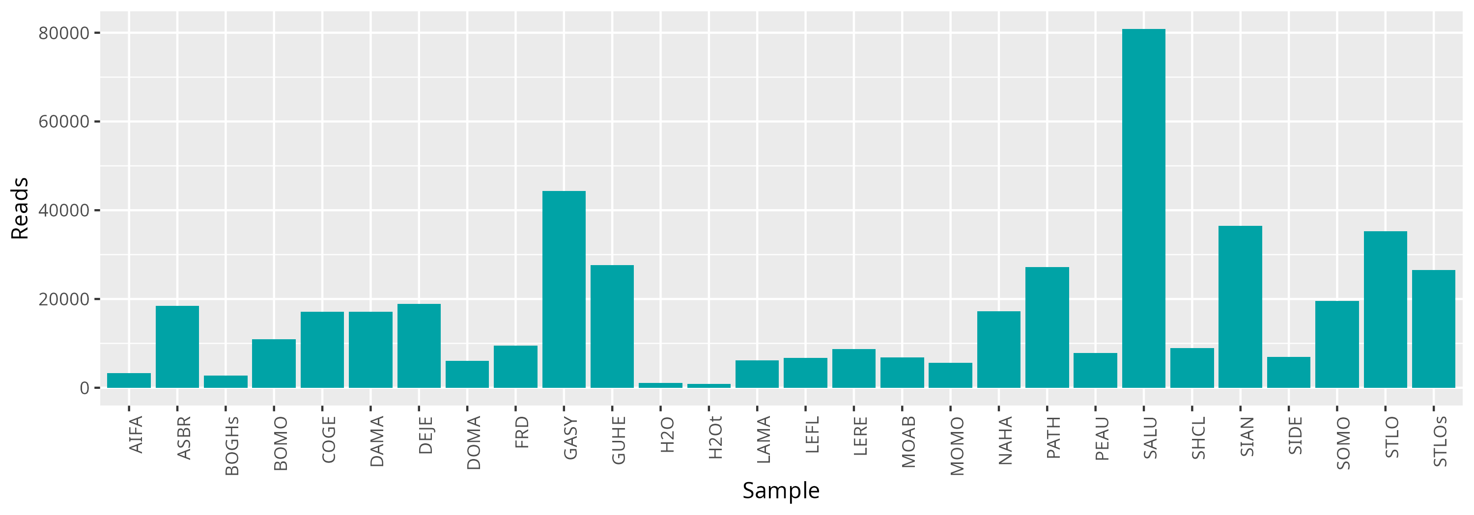
The information for all samples are indicated in the following table.

Warning

Some samples have very few reads. The sequencing effort may not be sufficient to detect a real signal

Quality control

The quality was assessed with FastQC [2] and MultiQC [3]. The aim of this step is to assess the quality of reads (per base quality, N content, length, adapter content…)

mkdir FASTQC LOGS
for i in RAW_DATA/*.fastq.gz ; do echo "conda activate fastqc-0.11.9 && fastqc $i -o FASTQC && conda deactivate" >> fastqc.sh ; done
qarray -cwd -V -N fastqc -o LOGS -e LOGS fastqc.sh
qsub -cwd -V -N multiqc -o LOGS -e LOGS -b y "conda activate multiqc-1.11 && multiqc FASTQC -o MULTIQC && conda deactivate"

Here is the MultiQC report. We can see that all reads have the same size (251). The sequence quality histograms are expected for Miseq sequencing. The adapter conent show high proportion for some samples (H20 and LEFL samples). It means the fragments were too small. Those reads will be discarded later.

Note

The quality of the sequencing, assessed by standard NGS tools, is good enough to process the data.

Bioinformatics

FROGS [4] is a tool dedicated to the analysis of large sets of DNA amplicons sequences accurately and rapidly. We used it to produce OTUs with taxonomic affiliations from raw reads.

Preprocess

The preprocess tool aims at cleaning and dereplicating sequences. Reads are merged with pear [5], primers are checked and removed with cutadapt [6], too small and too long sequences and with N inside are removed. Remaining sequences are finally dereplicated.

mkdir FROGS
cd FROGS
mkdir LOGS
qsub -cwd -V -N preprocess -o LOGS -e LOGS -pe thread 8 -R y -b y "conda activate frogs-4.0.1 && preprocess.py illumina --input-archive /work_home/orue/PMPBACT/RAW_DATA/PMPBACT.tar.gz --min-amplicon-size 200 --max-amplicon-size 490 --merge-software pear --five-prim-primer ACGGRAGGCAGCAG --three-prim-primer AGGATTAGATACCCTGGTA --R1-size 250 --R2-size 250 --nb-cpus 8 --output-dereplicated preprocess.fasta --output-count preprocess.tsv --summary preprocess.html --log-file preprocess.log && conda deactivate"

The preprocess report shows that ~93% of the reads overlap, have the expected size and do not have ambiguous bases. 392,585 sequences are remaining (from 470,880).

Clustering

The clustering tool uses swarm [7] to produce operation taxonomic units (OTUs) from sequences. We chose an aggregation distance of 1 (d=1). Swarm was developed to address two main issues of classical clustering methods (arbitrary global clustering thresholds, and input-order dependency induced by centroid selection) by first clustering nearly identical amplicons iteratively using a local threshold (d), and then by using clusters’ internal structure and amplicon abundances to refine its results.

qsub -cwd -V -N clustering -o LOGS -e LOGS -pe thread 8 -R y -b y "conda activate frogs-4.0.1 && clustering.py --input-fasta preprocess.fasta --input-count preprocess.tsv --distance 1 --fastidious --nb-cpus 8 --log-file clustering.log --output-biom clustering.biom --output-fasta clustering.fasta --output-compo clustering_otu_compositions.tsv && conda deactivate"
qsub -cwd -V -N clusters_stats -o LOGS -e LOGS -b y "conda activate frogs-4.0.1 && clusters_stat.py --input-biom clustering.biom --output-file clusters_stats.html --log-file clusters_stats.log && conda deactivate"

The clustering statistics report shows that the 392,585 sequences are grouped into 28,060 OTUs. 96% of the OTUs are composed of only 1 sequence and will be removed later. The biggest OTU is composed of 65,717 sequences.

Chimera removal

Chimeras are sequences formed from two or more biological sequences joined together. The majority of these anomalous sequences are formed from an incomplete extension during a PCR cycle. During subsequent cycles, a partially extended strand can bind to a template derived from a different but similar sequence. This phenomena is particularly common in amplicon sequencing where closely related sequences are amplified. The chimera detection is performed with vsearch [8].

qsub -cwd -V -N chimera -o LOGS -e LOGS -pe thread 8 -R y -b y "conda activate frogs-4.0.1 && remove_chimera.py --input-fasta clustering.fasta --input-biom clustering.biom --non-chimera remove_chimera.fasta --nb-cpus 8 --log-file remove_chimera.log --out-abundance remove_chimera.biom --summary remove_chimera.html && conda deactivate"

The specific report shows that 1.1% of the sequences are detected as chimeric sequences. It corresponds to 4% of the OTUs.

Filters on abundance

Here, we applied only a filter on abundance (not on prevalence). We applied the classical threshold of 0.005% of overall abundance (corresponding to 20 sequences). We checked also if phiX sequences still remain in sequences.

qsub -cwd -V -N filters -o LOGS -e LOGS -pe thread 8 -R y -b y "conda activate frogs-4.0.1 && otu_filters.py --input-fasta remove_chimera.fasta --input-biom remove_chimera.biom --output-fasta filters.fasta --nb-cpus 8 --log-file filters.log --output-biom filters.biom --summary filters.html --excluded filters_excluded.tsv --contaminant /db/outils/FROGS/contaminants/phi.fa --min-sample-presence 1 --min-abundance 0.00005 && conda deactivate"

The report shows that 186 OTUs are remaining (99.3% of OTUs are removed), corresponding to 360,732 sequences (92.9%). No phiX contamination is present. Everything is normal.

Taxonomic assignation

We now performed a taxonomic assignation of OTUs with blast [9] and Silva [10] (v. 138.1 pintail 100).

qsub -cwd -V -N affiliation -o LOGS -e LOGS -pe thread 8 -R y -b y "conda activate frogs-4.0.1 && affiliation_OTU.py --input-fasta filters.fasta --input-biom filters.biom --nb-cpus 8 --output-biom affiliation.biom --summary affiliation.html --reference /db/outils/FROGS/assignation/silva_138.1_16S_pintail100/silva_138.1_16S_pintail100.fasta && conda deactivate"
qsub -cwd -V -N affiliations_stats -o LOGS -e LOGS -b y "conda activate frogs-4.0.1 && affiliations_stat.py --input-biom affiliation.biom --output-file affiliations_stats.html --log-file affiliations_stats.log --multiple-tag blast_affiliations --tax-consensus-tag blast_taxonomy --identity-tag perc_identity --coverage-tag perc_query_coverage  && conda deactivate"

This report shows that 74% of the OTUs are affiliated (96% of sequences). 62% of the affiliated OTUs are multi-affiliated at Species level (the sequence may be not discriminating enough to differentiate between several species of the same genus). The alignment distribution tab in this report shows that blast hits demonstrate all a high identity and coverage percents, except 2 with 6676 sequences. The affiliation of these OTUs have to be checked.

Note

Species can not be assigned for a lot of OTUs. It is expected for 16S sequences because 16S rRNA sequence is often the same between Species.

Finally, we created a TSV file from the BIOM file.

qsub -cwd -V -N biom_to_tsv -o LOGS -e LOGS -b y "conda activate frogs-4.0.1 && biom_to_tsv.py --input-biom affiliation.biom --input-fasta filters.fasta --output-tsv affiliation.tsv --output-multi-affi multi_aff.tsv --log-file biom_to_tsv.log  && conda deactivate"

Informations are displayed in the following table:

Some sequences were not affiliated against Silva. We checked manually from the NCBI blast website their taxonomic affiliation. An example is available in the following screenshot. OTUs without affiliation are human or mouse sequences.

Figure 2: Taxonomic affiliation of a previously unaffiliated OTU sequence

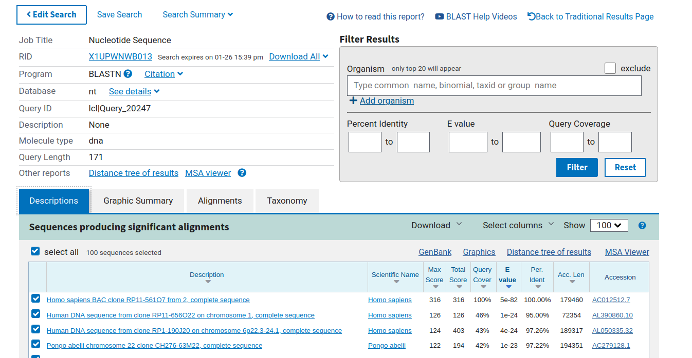
We removed them with the otu_filters tool (we chose the human genome as contaminant) and checked the result.

qsub -cwd -V -N filters -o LOGS -e LOGS -pe thread 8 -R y -b y "conda activate frogs-4.0.1 && otu_filters.py --contaminant hs1.fa --input-biom affiliation.biom --input-fasta filters.fasta --output-biom affiliation2.biom --output-fasta filters2.fasta --summary filters2.html --log-file filters2.log --excluded filters2_excluded.tsv && conda deactivate"
qsub -cwd -V -N affiliations_stats2 -o LOGS -e LOGS -b y "conda activate frogs-4.0.1 && affiliations_stat.py --input-biom affiliation2.biom --output-file affiliations_stats2.html --log-file affiliations_stats2.log --multiple-tag blast_affiliations --tax-consensus-tag blast_taxonomy --identity-tag perc_identity --coverage-tag perc_query_coverage  && conda deactivate"

The updated report shows that some OTUs without affiliation are still present. They (Cluster_117, Cluster_115, Cluster_202, Cluster_214, Cluster_67, CLuster_111) are human and mouse sequences. We have removed them later.

Here are the multiple affiliations found for each multi-affiliated OTU:

Tip

AffiliationExplorer can be used to easily deal with multi-affiliations. The aim is to check if some multi-affiliations could be corrected.

Phylogenetic tree

We built a phylogenetic tree by performing a multiple alignment of OTUs with Mafft [11] and then by creating a rooted phylogenetic tree with FastTree [12] and the Phangorn R package [13].

qsub -cwd -V -N tree -o LOGS -e LOGS -pe thread 8 -R y -b y "conda activate frogs-4.0.1 &&tree.py --input-sequences filters2.fasta --biom-file affiliation2.biom --out-tree tree.nwk && conda deactivate"

Biostatistics

We used phyloseq [14]. The phyloseq package is a tool to import, store, analyze, and graphically display complex phylogenetic sequencing data that has already been clustered into Operational Taxonomic Units (OTUs), especially when there is associated sample data, phylogenetic tree, and/or taxonomic assignment of the OTUs.

Here are the informations about the samples:

Table 1: Metadata of samples

sample	Host	Column	Grade	Sex	Age	PCI
STLOs	souris	1	HG	NA	NA	NA
BOGHs	souris	1	HG	NA	NA	NA
DOMA	humain	1	HG	F	69	NA
STLO	humain	1	HG	M	NA	NA
PATH	humain	1	HG	M	47	NA
GUHE	humain	1	HG	M	64	39
GASY	humain	1	HG	F	52	NA
SOMO	humain	1	HG	F	72	NA
MOAB	humain	2	BG	M	43	30
SALU	humain	2	BG	F	58	NA
SIAN	humain	2	BG	M	NA	NA
DEJE	humain	2	BG	M	50	NA
COGE	humain	2	BG	M	62	NA
LAMA	humain	2	BG	F	83	NA
PEAU	humain	2	BG	F	43	NA
LERE	humain	2	BG	M	73	39
ASBR	humain	3	BG	M	57	NA
LEFL	humain	3	HG	F	43	NA
DAMA	humain	3	BG	F	68	NA
SIDE	humain	3	BG	F	55	NA
BOMO	humain	3	BG	F	NA	NA
SHCL	humain	3	BG	F	56	NA
MOMO	humain	3	NA	M	72	NA
AIFA	humain	3	BG	F	62	NA
NAHA	humain	4	BG	M	46	NA
FRD	humain	4	BG	F	NA	NA
H2O	control	12	NA	NA	NA	NA
H2Ot	control	12	NA	NA	NA	NA

We removed OTUs without affiliations.

my_bad_otus <- c("Cluster_117", "Cluster_115", "Cluster_202", "Cluster_214", "Cluster_67", "Cluster_111")
allTaxa = taxa_names(physeq)
allTaxa_final <- allTaxa[!(allTaxa %in% my_bad_otus)]
physeq <- prune_taxa(allTaxa_final, physeq)

6 OTUs have been removed.

Finally, we checked the amount of reads lost before and after all our analyses.

Figure 3: Reads before and after bioinformatics.

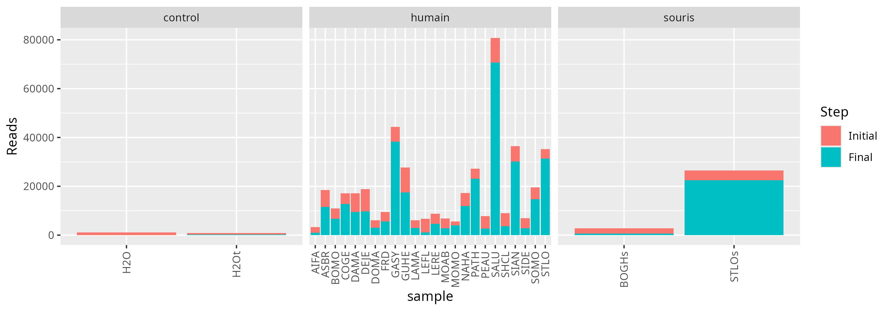
Note

Globally, 72.11% of reads is present in our count table.

Control samples

Let look at the composition of the control samples. The composition is different between them but represent very few reads. We can remove them.

physeq_controls <- subset_samples(physeq, Host=="control")
p <- plot_composition(physeq = physeq_controls, taxaRank1 = "Kingdom", taxaSet1 = "Bacteria", taxaRank2 = "Phylum", numberOfTaxa = 10L, x = "Sample")
physeq <- subset_samples(physeq, Host!="control")

This is what our phyloseq object is made of:

physeq

phyloseq-class experiment-level object
otu_table()   OTU Table:         [ 138 taxa and 26 samples ]
sample_data() Sample Data:       [ 26 samples by 8 sample variables ]
tax_table()   Taxonomy Table:    [ 138 taxa by 7 taxonomic ranks ]
phy_tree()    Phylogenetic Tree: [ 138 tips and 137 internal nodes ]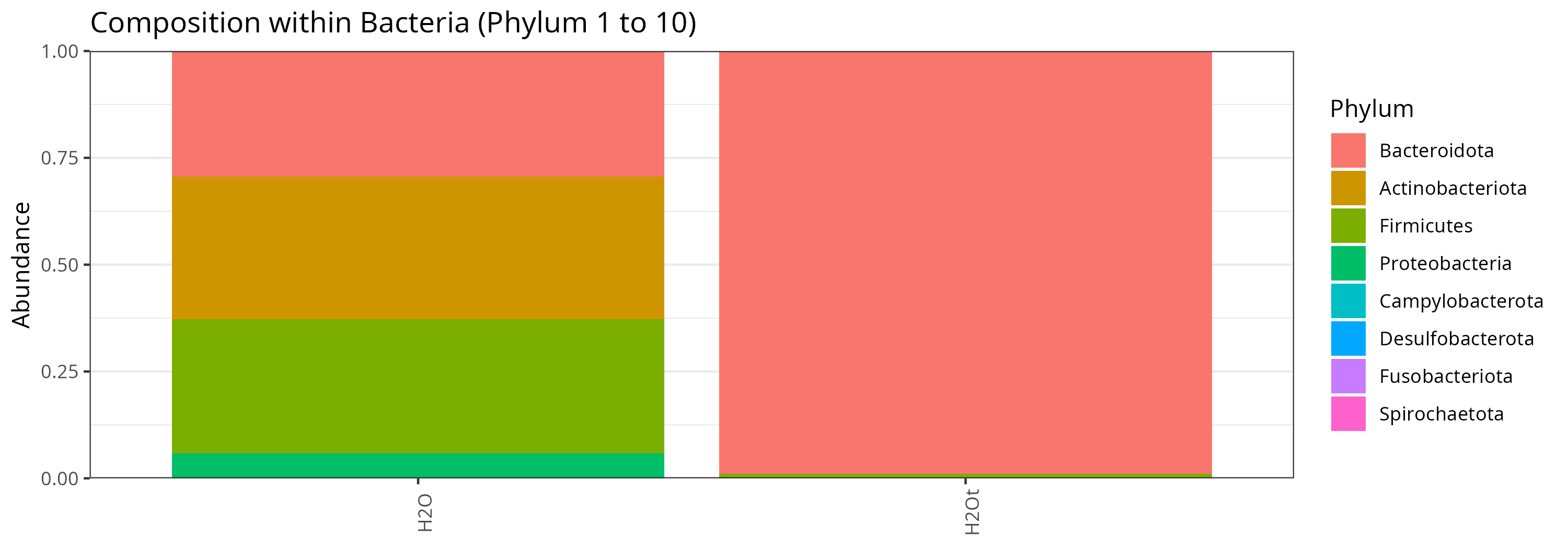

Figure 4: Rarefaction curves.

The final phyloseq object is avaialble here

Rarefaction curves

The depth is not homogenous between samples.

sample_sums(physeq) %>% sort()

BOGHs  AIFA  LEFL  PEAU  SIDE  MOAB  LAMA  DOMA  SHCL  MOMO  LERE   FRD  BOMO 
  621  1038  1145  2644  2744  2799  2867  3094  3633  3961  4679  5549  6672 
 DAMA  DEJE  ASBR  NAHA  COGE  SOMO  GUHE STLOs  PATH  SIAN  STLO  GASY  SALU 
 9506  9771 11565 11904 12703 14684 17469 22515 23033 30080 31398 38229 70692 

and the rarefaction curves demonstrate it.

We test whether the depths used in this study are sufficient to capture the microbial diversity. The rarefaction do not reach a flat plateau for the majority of samples.

p <- ggrare(physeq, step = 500, se = FALSE, color = "Host", plot = FALSE, verbose = FALSE)
p <- p + geom_vline(xintercept = c(min(sample_sums(physeq)), 5000), 
               color = "grey50", linetype = "dashed") +
  facet_grid(~ Host)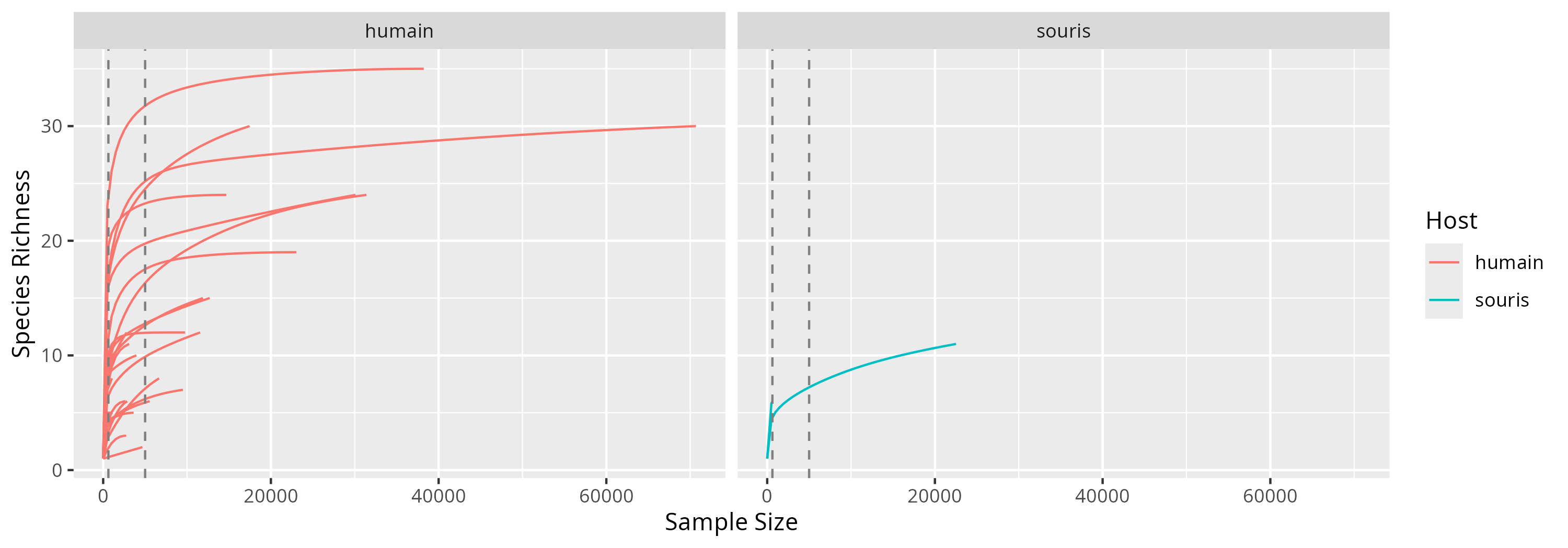

Figure 5: Rarefaction curves.

The shallowest samples clearly have too few reads to reflect the whole composition.

Alpha diversity

The observed richness is between a few OTUs and about 30.

p <- plot_richness(physeq = physeq, x = "samples", color = "Host", shape = NULL, title = "Alpha diversity graphics", measures = c("Observed"))
p <- p + geom_boxplot() + geom_point()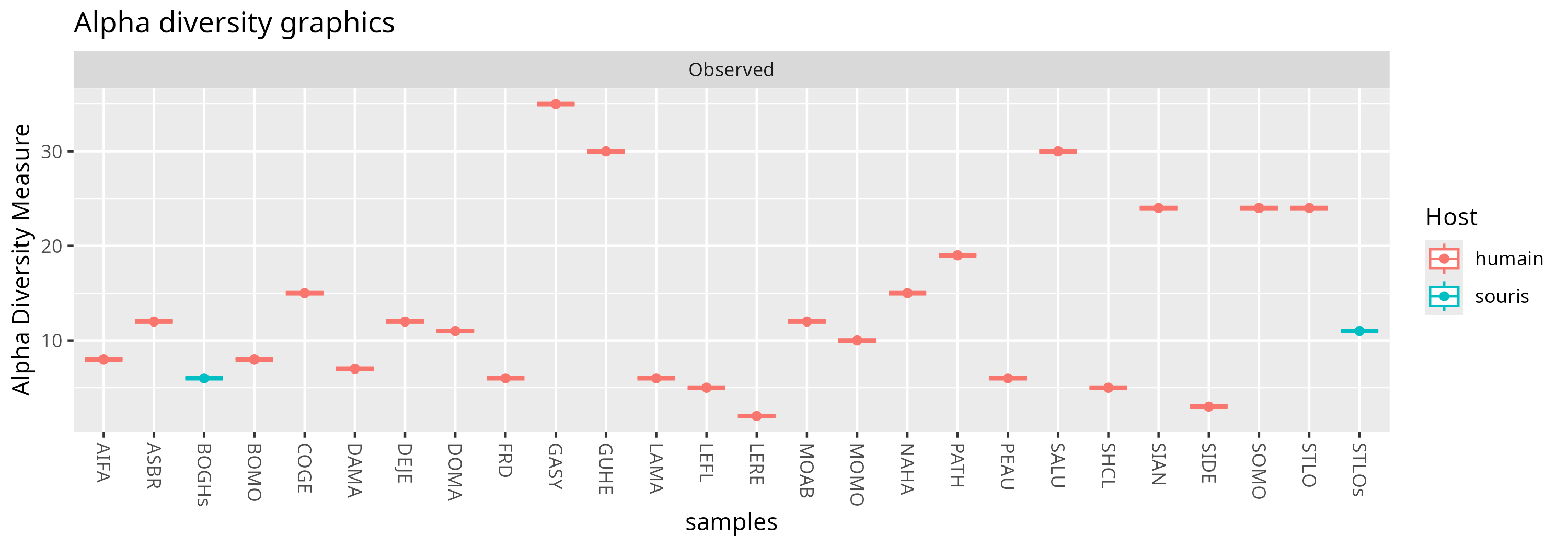 

Figure 6: Observed richness accross samples.

Compositions

We can look at the composition at the Phylum level

p <- plot_composition(physeq = physeq, taxaRank1 = "Kingdom", taxaSet1 = "Bacteria", taxaRank2 = "Phylum", numberOfTaxa = 10L, x = "Sample", title = "")
p <- p + facet_grid(". ~ Host", scales = "free_x", space = "free")

Figure 7: Composition at Phylum level

The samples composition is very different according to samples, even inside Human/Mouse samples.

Tip

To go further, Easy16S can be used with the rds file available in the Downloads section to explore in depth the results.

Downloads

• RDS file
• Multi-affiliation file
• TSV file containing counts and affiliation of OTUs

References

Figure 1: Raw reads number per sample. Figure 2: Taxonomic affiliation of a previously unaffiliated OTU sequence Figure 3: Reads before and after bioinformatics. Figure 4: Rarefaction curves. Figure 5: Rarefaction curves. Figure 6: Observed richness accross samples. Figure 7: Composition at Phylum level

References

1. Shen W, Le S, Li Y, Hu F. SeqKit: A cross-platform and ultrafast toolkit for FASTA/q file manipulation. PloS one. 2016;11:e0163962.

2. Andrews S. FastQC a quality control tool for high throughput sequence data. http://www.bioinformatics.babraham.ac.uk/projects/fastqc/. 2010. http://www.bioinformatics.babraham.ac.uk/projects/fastqc/.

3. Ewels P, Magnusson M, Lundin S, Käller M. MultiQC: Summarize analysis results for multiple tools and samples in a single report. Bioinformatics. 2016;32:3047–8.

4. Escudié F, Auer L, Bernard M, Mariadassou M, Cauquil L, Vidal K, et al. FROGS: Find, Rapidly, OTUs with Galaxy Solution. Bioinformatics. 2018;34:1287–94. doi:10.1093/bioinformatics/btx791.

5. Zhang J, Kobert K, Flouri T, Stamatakis A. PEAR: A fast and accurate illumina paired-end reAd mergeR. Bioinformatics. 2013;30:614–20.

6. Martin M. Cutadapt removes adapter sequences from high-throughput sequencing reads. EMBnet journal. 2011;17:10–2.

7. Mahé F, Rognes T, Quince C, Vargas C de, Dunthorn M. Swarm v2: Highly-scalable and high-resolution amplicon clustering. PeerJ. 2015;3:e1420.

8. Rognes T, Flouri T, Nichols B, Quince C, Mahé F. VSEARCH: A versatile open source tool for metagenomics. PeerJ. 2016;4:e2584.

9. Altschul SF, Gish W, Miller W, Myers EW, Lipman DJ. Basic local alignment search tool. Journal of molecular biology. 1990;215:403–10.

10. Quast C, Pruesse E, Yilmaz P, Gerken J, Schweer T, Yarza P, et al. The SILVA ribosomal RNA gene database project: Improved data processing and web-based tools. Nucleic acids research. 2012;41:D590–6.

11. Katoh K, Standley DM. MAFFT multiple sequence alignment software version 7: Improvements in performance and usability. Molecular biology and evolution. 2013;30:772–80.

12. Price MN, Dehal PS, Arkin AP. FastTree 2–approximately maximum-likelihood trees for large alignments. PloS one. 2010;5:e9490.

13. Schliep KP. Phangorn: Phylogenetic analysis in r. Bioinformatics. 2011;27:592–3.

14. McMurdie PJ, Holmes S. Phyloseq: An r package for reproducible interactive analysis and graphics of microbiome census data. PloS one. 2013;8:e61217.