Show the code
#Use packages and functions
library(tidyverse)
library(edgeR)
library(ggplot2)
library(kableExtra)
library(ExperimentSubset)
library(colorspace)
library(openxlsx) # manipulation excel files
#sessionInfo()Experiment with BA
#Use packages and functions
library(tidyverse)
library(edgeR)
library(ggplot2)
library(kableExtra)
library(ExperimentSubset)
library(colorspace)
library(openxlsx) # manipulation excel files
#sessionInfo()We used datasets created at the exploration and normalisation step from BA experiment. Genes with too low expression were filtered. A normalization factor is calculated to take into account the different sizes of the sequencing banks (i.e. the total read count) and the distribution of reads per sample on sequencing run, as discussed [1]. Read counts were normalized using trimmed mean of M-values (TMM) method [2] from edgeR
# load a dge object
dge_ofinterest <- paste("../output/Restorbiome_dge_", params$my.interest, ".rds", sep="")
dge <- readRDS(dge_ofinterest)
# print(dge)
head(dge$counts, n=3)
BA_G_R1 BA_G_R2 BA_G_R3 BA_R_R1 BA_R_R2 BA_R_R3
gene-BAD_RS00005 6201 4936 4267 3441 2897 3652
gene-BAD_RS00010 6815 5705 4232 8147 5974 7703
gene-BAD_RS00015 1956 1488 1078 1824 1403 1736Above an extract from the expression matrix which contains expression on 1713 expressed genes and 6 samples from BA experiment.
The aim is to identify the genes differentially expressed between treatment and Glucose.
The differential analysis is based on a Generalized Linear Model (GLM) to take into account the distribution of count-type data (non-normality of the data) and over-dispersion. The regression coefficients of the factors are estimated by a log-linear model.
Using edgeR
dge$samples$group <- as.factor(dge$samples$group)
dge$samples$group <- relevel(dge$samples$group, ref = paste(params$my.interest, "G", sep="_"))
# levels(dge$samples$group)

#matrix design: one factor group
design <- model.matrix(~ 0 + group, data = dge$samples)
colnames(design) <- gsub(paste0("group", params$my.interest, "_"), "", colnames(design))
# design#--- make all contrasts of interest
# treatment versus control condition
RvsG <- makeContrasts(R-G, levels=colnames(design))
my.contrasts <- list(RvsG = RvsG)
names(my.contrasts) <- paste(params$my.interest, names(my.contrasts), sep="_")We set robust=TRUE when estimating the dispersion. This has no effect on the downstream analysis, but is nevertheless very useful for identifying outliers from the trend of the mean dispersion of the negative binomial distribution.
# robust at gene level
# with specific design
dge<-estimateDisp(dge, design = design, robust=TRUE)
#summary(dge$tagwise.dispersion)
plotBCV(dge)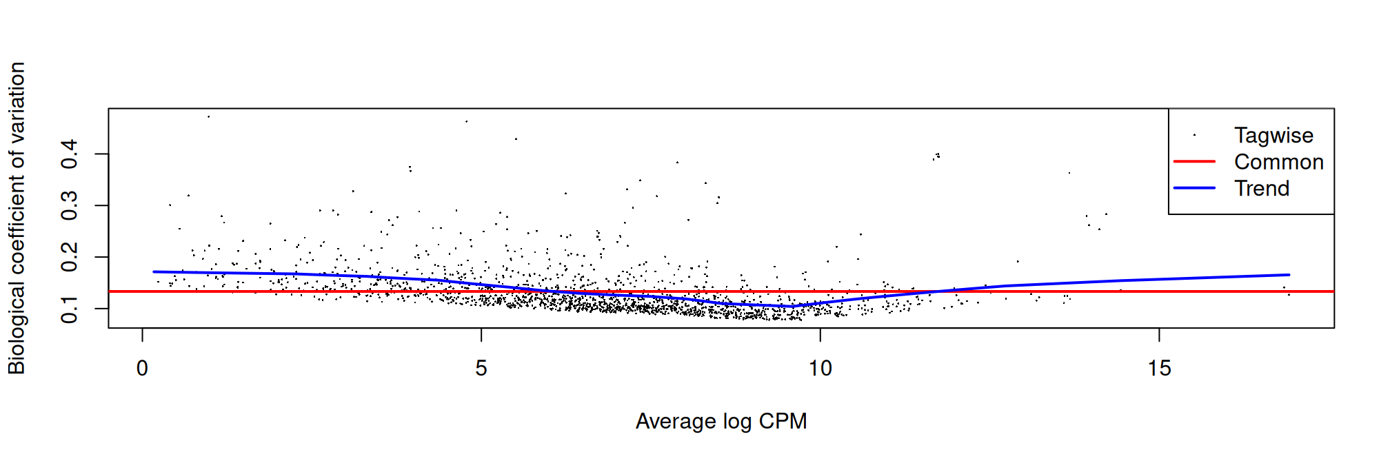
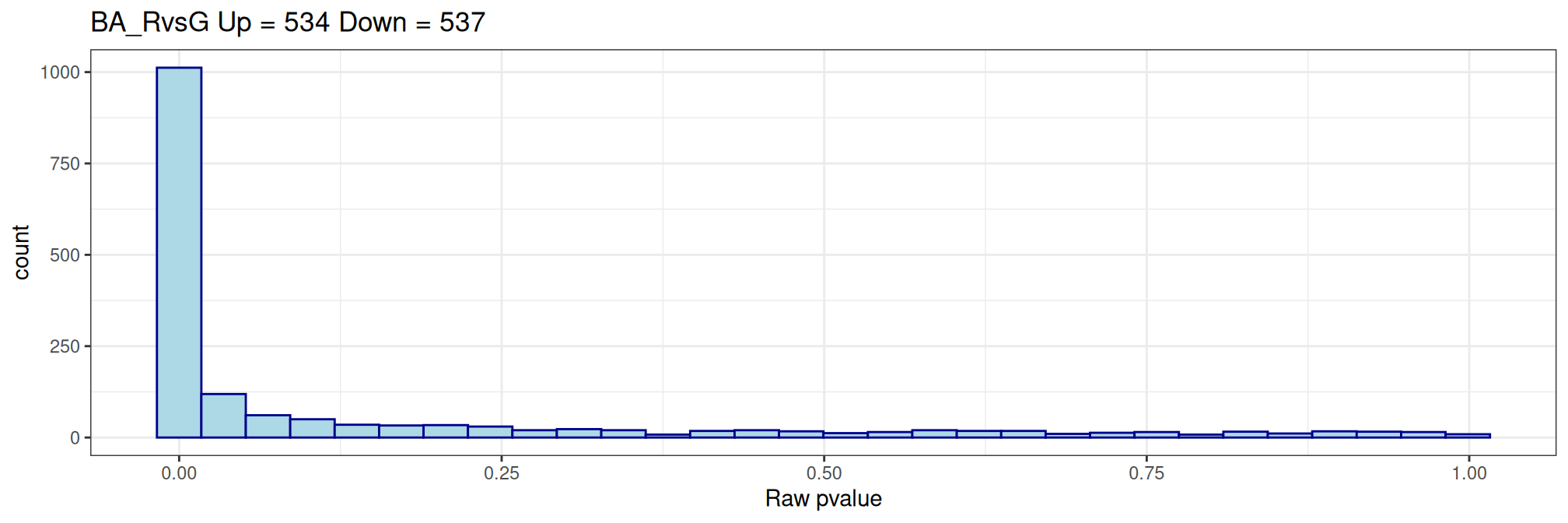
We used GLM model [3] to perform likelihood ratio tests for each contrast defined as treatment versus Glucose control treatment. List of differentially expressed genes were obtained after controlling the false discovery rate with a Benjamini-Hochberg correction [4] at 0.05 threshold.
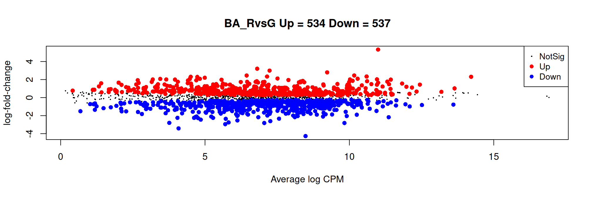
Histogram of raw p-values and mean-difference plot (also called MA-plot) are useful graphs to validate the model.
#only the trended dispersion is used under the QL
method <- "LRT"
#fit <- glmFit(dge, dge$design)
#  with specific design
fit <- glmFit(dge, design = design)
#head(fit$coefficients)
#head(fit$dispersion)
res<-list()
nDiffTotal <- NULL

#fit model for each contrast
for (ctr in 1:length(my.contrasts)){
 qlf<- glmLRT(fit, contrast = my.contrasts[[ctr]])
 topTags(qlf)
 # Results, Nb of DE
 #cat("contrast= ",names(my.contrasts)[ctr],"\n")
 #print(summary(decideTestsDGE(qlf)))
 nDiffTotal <- cbind(nDiffTotal, summary(decideTestsDGE(qlf)))
 # results of tests
 res[[ctr]]<-topTags(qlf,n=nrow(dge$counts),adjust.method="BH",sort.by="none")$table
 names(res)[ctr]<-names(my.contrasts)[ctr]
 # histogram of raw pvalues
 my.title <- paste(names(my.contrasts)[ctr], "Up =", nDiffTotal[,ctr]["Up"], "Down =", nDiffTotal[,ctr]["Down"])
 p <- ggplot(data = qlf$table, aes(x = PValue))
 p <- p + geom_histogram(color="darkblue", fill="lightblue")
 p <- p + theme_bw() + xlab("Raw pvalue")
 p <- p + ggtitle(my.title)
 print(p)
 # MA plot
 plotMD(qlf, main = my.title)
}
# results combined in a list object
# initialisation

#--- summary number of DE by contrast
nDiffTotal <- as.data.frame(nDiffTotal)
colnames(nDiffTotal) <- names(my.contrasts)
cat("\nNumber of features down/up and total:\n")
Number of features down/up and total:nDiffTotal %>% kbl() %>% kable_styling() %>% scroll_box(width = "100%", height = "200px")| BA_RvsG | |
|---|---|
| Down | 537 |
| NotSig | 642 |
| Up | 534 |
# write.table(nDiffTotal,
#             file = paste("../output/2_Differential_Analysis",params$my.interest,".resume.xls", sep=""),
#             sep = "\t", row.names = TRUE,
# dec = ".", quote = FALSE)# List of DE result from each contrast as a dataframe with informations like logFC, PValue, FDR...
saveRDS(res, file=paste("../output/Restorbiome_DE_", params$my.interest,".rds",sep=""))sessioninfo::session_info(pkgs = "attached")─ Session info ───────────────────────────────────────────────────────────────
setting value
version R version 4.4.2 (2024-10-31)
os Ubuntu 24.04.1 LTS
system x86_64, linux-gnu
ui X11
language (EN)
collate fr_FR.UTF-8
ctype fr_FR.UTF-8
tz Europe/Paris
date 2025-02-16
pandoc 3.1.1 @ /usr/lib/rstudio/resources/app/bin/quarto/bin/tools/ (via rmarkdown)
─ Packages ───────────────────────────────────────────────────────────────────
package * version date (UTC) lib source
Biobase * 2.64.0 2024-04-30 [1] Bioconductor 3.19 (R 4.4.0)
BiocGenerics * 0.50.0 2024-04-30 [1] Bioconductor 3.19 (R 4.4.0)
Biostrings * 2.72.1 2024-06-02 [1] Bioconductor 3.19 (R 4.4.0)
colorspace * 2.1-1 2024-07-26 [1] CRAN (R 4.4.0)
dplyr * 1.1.4 2023-11-17 [1] CRAN (R 4.4.0)
edgeR * 4.2.2 2024-10-13 [1] Bioconductor 3.19 (R 4.4.1)
ExperimentSubset * 1.14.0 2024-04-30 [1] Bioconductor 3.19 (R 4.4.2)
forcats * 1.0.0 2023-01-29 [1] CRAN (R 4.4.0)
GenomeInfoDb * 1.40.1 2024-05-24 [1] Bioconductor 3.19 (R 4.4.0)
GenomicRanges * 1.56.2 2024-10-09 [1] Bioconductor 3.19 (R 4.4.1)
ggplot2 * 3.5.1 2024-04-23 [1] CRAN (R 4.4.0)
IRanges * 2.38.1 2024-07-03 [1] Bioconductor 3.19 (R 4.4.1)
kableExtra * 1.4.0 2024-01-24 [1] CRAN (R 4.4.0)
limma * 3.60.6 2024-10-02 [1] Bioconductor 3.19 (R 4.4.1)
lubridate * 1.9.4 2024-12-08 [1] CRAN (R 4.4.2)
MatrixGenerics * 1.16.0 2024-04-30 [1] Bioconductor 3.19 (R 4.4.0)
matrixStats * 1.5.0 2025-01-07 [1] CRAN (R 4.4.2)
openxlsx * 4.2.8 2025-01-25 [1] CRAN (R 4.4.2)
purrr * 1.0.2 2023-08-10 [1] CRAN (R 4.4.0)
readr * 2.1.5 2024-01-10 [1] CRAN (R 4.4.0)
S4Vectors * 0.42.1 2024-07-03 [1] Bioconductor 3.19 (R 4.4.1)
SingleCellExperiment * 1.26.0 2024-04-30 [1] Bioconductor 3.19 (R 4.4.2)
SpatialExperiment * 1.14.0 2024-05-01 [1] Bioconductor 3.19 (R 4.4.2)
stringr * 1.5.1 2023-11-14 [1] CRAN (R 4.4.0)
SummarizedExperiment * 1.34.0 2024-05-01 [1] Bioconductor 3.19 (R 4.4.0)
tibble * 3.2.1 2023-03-20 [1] CRAN (R 4.4.0)
tidyr * 1.3.1 2024-01-24 [1] CRAN (R 4.4.0)
tidyverse * 2.0.0 2023-02-22 [1] CRAN (R 4.4.0)
TreeSummarizedExperiment * 2.12.0 2024-04-30 [1] Bioconductor 3.19 (R 4.4.2)
XVector * 0.44.0 2024-04-30 [1] Bioconductor 3.19 (R 4.4.0)
[1] /home/orue/R/x86_64-pc-linux-gnu-library/4.4
[2] /usr/local/lib/R/site-library
[3] /usr/lib/R/site-library
[4] /usr/lib/R/library
──────────────────────────────────────────────────────────────────────────────A work by Migale Bioinformatics Facility
Université Paris-Saclay, INRAE, MaIAGE, 78350, Jouy-en-Josas, France
Université Paris-Saclay, INRAE, BioinfOmics, MIGALE bioinformatics facility, 78350, Jouy-en-Josas, France