#Use packages and functionslibrary(tidyverse)library(data.table)library(SummarizedExperiment) # manipulation RNASeq assayslibrary(rtracklayer) ## for annotation#library("DEFormats")library(edgeR)library(kableExtra)library(dplyr)library(purrr)library(stringr)library(ggplot2)library(reshape2)library(mixOmics) #PCA
Read counts
The matrix of raw counts looks like that.
Show the code
#cat("EXP = ", params$my.interest)### Get Raw Count data in edgeR object# At gene level#inputFile <- "count_allSamples_BA.csv"inputFile <-list.files("../data/counts") |>str_subset(params$my.interest)#cat("File raw = ",inputFile,"\n")rawdata <-fread(file.path("../data/counts",inputFile))# rename first column gene ID to be homogenous between assayscolnames(rawdata)[1] <-"Gene_ID"nameEXP <- params$my.interest# genecount: count matrixgeneCount <- rawdata[,-c(1)] |>as.matrix()row.names(geneCount) <- rawdata %>% dplyr::select(1) %>%unlist() %>%as.character()#row.names(geneCount) %>% head()#print(dim(geneCount))head(geneCount) %>%kbl() %>%kable_styling() %>%scroll_box(width ="100%", height ="200px")
BA_G_R1
BA_G_R2
BA_G_R3
BA_R_R1
BA_R_R2
BA_R_R3
gene-BAD_RS00005
6201
4936
4267
3441
2897
3652
gene-BAD_RS00010
6815
5705
4232
8147
5974
7703
gene-BAD_RS00015
1956
1488
1078
1824
1403
1736
gene-BAD_RS00020
533
441
273
635
401
525
gene-BAD_RS00025
8473
5992
4906
3805
2754
3120
gene-BAD_RS00030
17965
12906
11256
5707
3939
4261
This matrix contains raw counts from BA experiment with 1729 genes and 6 samples.
# GFF annotation filefilegff <-case_when( nameEXP =='BA'~"../data/GFF/NC_008618_bifido_adolescentis_spikes_cazymes_dbcan.gff3", nameEXP =='BU'~"../data/GFF/CP102263_1_Bacteroides_uniformis_spikes_cazymes_dbcan_pulpred_cc.gff3", nameEXP =='BC'~"../data/GFF/NZ_AP012325_bifido_catenulatum_spikes_cazymes_dbcan.gff3", nameEXP =='ER'~"../data/GFF/NC_012781_eubacterium_rectale_spikes_cazymes_dbcan.gff3",)# use gff produced by DBCANgff <-readGFF(filegff)df_annot <- gff %>%as_tibble() %>%unnest_longer(Parent) # remove comulmn with all NAdf_annot <- df_annot %>%select_if(~sum(!is.na(.)) >0) # Remark: duplicated gene annotation# which(duplicated(df_annot[,"Parent"]))# keeep the first line when multiple annotationdf_annot <- df_annot%>%group_by(seqid, source, type, ID, Parent) %>%filter(row_number() <=1)#glimpse(df_annot)rawdata_annot <-left_join(rawdata[, 1], df_annot, by=c("Gene_ID"="Parent"), keep=FALSE) %>%as.data.frame()#glimpse(rawdata_annot)
In this BA experiment, the effect of each treatment (G, R) on gene expression will be explore. The number of biological repetitions is 3, 3 for G, R treatment, respectively.
Genes with very low counts across all libraries may be filtered.
Show the code
# Filter gene with low count, at least number of biological replicates with cpm > valfilt #summary(libsize)#valfilt <- round(10*1e06 / min(libsize), 1)valfilt <-1nbrepbio <-min(table(colData(se)$group))keep <-rowSums(edgeR::cpm(se) > valfilt) >= nbrepbio#summary(keep)se <- se[keep,]#dim(se)
The filtering on genes is based on count per million (cpm) greater than 1 in at least 3 samples corresponding to the minimum number of biological replicates. We kept 1713 expressed genes for further analyses from 6 samples.
Normalisation
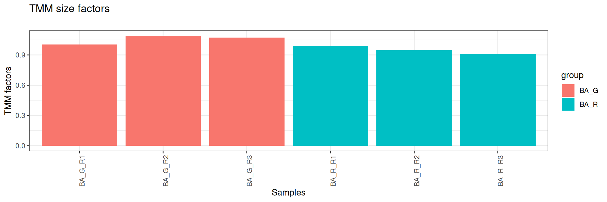
A normalization factor is calculated to take into account the different sizes of the sequencing banks (i.e. the total read count) and the distribution of reads per sample on sequencing run, as discussed [1]. Normalization by trimmed mean of M values (TMM) [2] is performed by using the calcNormFactors function from edgeR R package. It calculates a set of normalization factors, one for each sample, to eliminate composition biases between libraries.
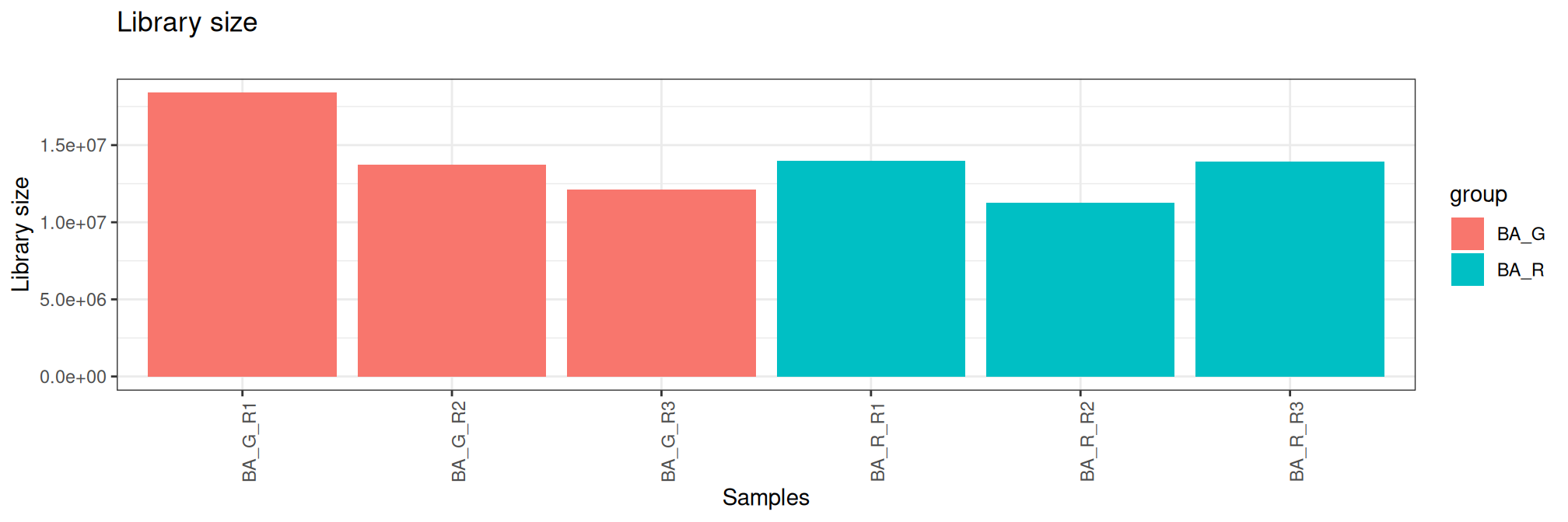
Here, the table contains library size and normalisation factors using TMM method ordered by library size. These graphs are another way of verifying the quality control carried out during the sequencing and bioinformatics analysis steps.
        group lib.size norm.factors Bacteria Treatment Replicate  sample
BA_R_R2  BA_R 11288923    0.9468454       BA         R        R2 BA_R_R2
BA_G_R3  BA_G 12108903    1.0737004       BA         G        R3 BA_G_R3
BA_G_R2  BA_G 13758228    1.0889577       BA         G        R2 BA_G_R2
BA_R_R3  BA_R 13912355    0.9092578       BA         R        R3 BA_R_R3
BA_R_R1  BA_R 13997036    0.9886040       BA         R        R1 BA_R_R1
BA_G_R1  BA_G 18392123    1.0048875       BA         G        R1 BA_G_R1
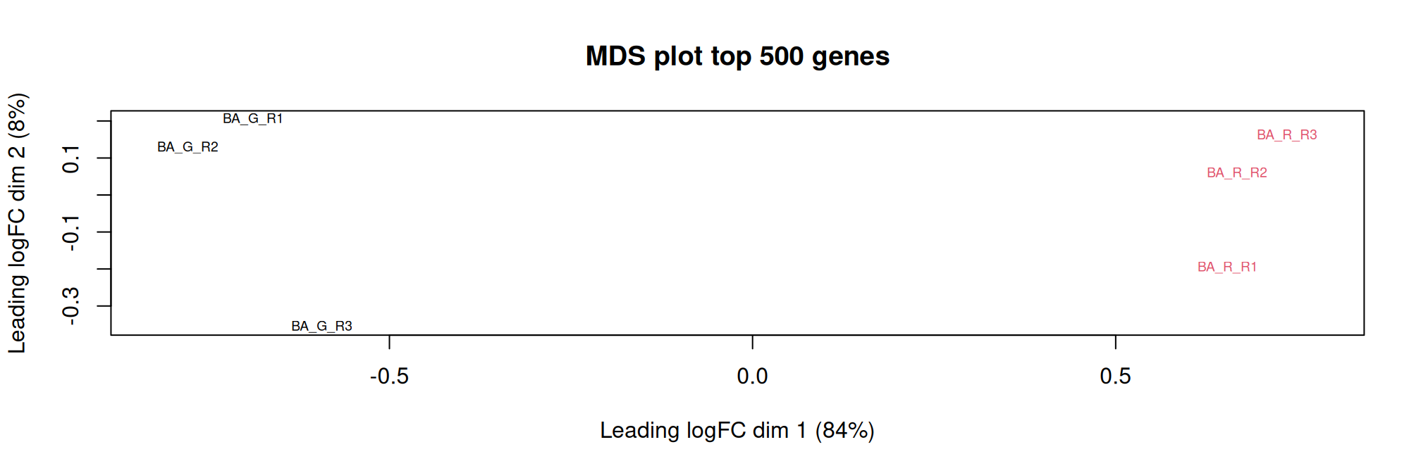
Multidimensional scaling (MDS) plot shows the relationships between the samples. The top (500 genes) are used to calculate the distance between expression profiles of samples. The distance approximate the log2 fold change between the samples.
As expected, samples are grouped by treatment.
Show the code
limma::plotMDS(dge, col =as.numeric(dge$samples$group), labels = dge$samples$sample, cex=0.6, top =500, main ="MDS plot top 500 genes")
1. Dillies M-A, Rau A, Aubert J, Hennequet-Antier C, Jeanmougin M, Servant N, et al. A comprehensive evaluation of normalization methods for illumina high-throughput RNA sequencing data analysis. Brief Bioinform. 2012;14:671–83.
2. Robinson MD, Oshlack A. A scaling normalization method for differential expression analysis of RNA-seq data. Genome Biology. 2010;11:R25. doi:10.1186/gb-2010-11-3-r25.
Reuse
This document will not be accessible without prior agreement of the partners
A work by Migale Bioinformatics Facility
Université Paris-Saclay, INRAE, MaIAGE, 78350, Jouy-en-Josas, France
Université Paris-Saclay, INRAE, BioinfOmics, MIGALE bioinformatics facility, 78350, Jouy-en-Josas, France
Source Code
---params: my.interest: "BU"title: "RESTORBIOME2: Exploration and normalisation"subtitle: "Experiment with `r params$my.interest`"author: - name: Olivier Rué orcid: 0000-0003-1689-0557 email: olivier.rue@inrae.fr affiliations: - name: Migale bioinformatics facility adress: Domaine de Vilvert city: Jouy-en-Josas state: France - name: Christelle Hennequet-Antier orcid: 0000-0001-5836-2803 email: christelle.hennequet-antier@inrae.fr affiliations: - name: Migale bioinformatics facility adress: Domaine de Vilvert city: Jouy-en-Josas state: Francedate: "2023-05-02"date-modified: today#bibliography: ../../../resources/biblio.bib # don't change#csl: ../../../resources/biomed-central.csl # don't change# # Do not modify this section without taking precautions# # Don't remove the commented line, it is usefull for building the site with this new project!license: "This document will not be accessible without prior agreement of the partners"format: html: embed-resources: false toc: true toc-location: right page-layout: article code-overflow: wrap code-fold: true code-tools: true code-summary: "Show the code"---```{r}#| label = "setup",#| include = FALSEknitr::opts_chunk$set(echo =TRUE, cache =FALSE, message =FALSE, warning =FALSE, fig.height =3.5, fig.width =10.5)``````{r}#| label = "setuplib"#Use packages and functionslibrary(tidyverse)library(data.table)library(SummarizedExperiment) # manipulation RNASeq assayslibrary(rtracklayer) ## for annotation#library("DEFormats")library(edgeR)library(kableExtra)library(dplyr)library(purrr)library(stringr)library(ggplot2)library(reshape2)library(mixOmics) #PCA```# Read countsThe matrix of raw counts looks like that.```{r}#| label = "LoadRawdata"#cat("EXP = ", params$my.interest)### Get Raw Count data in edgeR object# At gene level#inputFile <- "count_allSamples_BA.csv"inputFile <-list.files("../data/counts") |>str_subset(params$my.interest)#cat("File raw = ",inputFile,"\n")rawdata <-fread(file.path("../data/counts",inputFile))# rename first column gene ID to be homogenous between assayscolnames(rawdata)[1] <-"Gene_ID"nameEXP <- params$my.interest# genecount: count matrixgeneCount <- rawdata[,-c(1)] |>as.matrix()row.names(geneCount) <- rawdata %>% dplyr::select(1) %>%unlist() %>%as.character()#row.names(geneCount) %>% head()#print(dim(geneCount))head(geneCount) %>%kbl() %>%kable_styling() %>%scroll_box(width ="100%", height ="200px")```This matrix contains raw counts from `r params$my.interest` experiment with `r nrow(geneCount)` genes and `r ncol(geneCount)` samples.This is the experimental design.```{r}#| label = "Design"# create Design from sample's names in filesampleInfo.all <-colnames(rawdata)[-c(1)] %>% stringr::str_split(., "[_]", simplify =FALSE) %>%transpose() %>% purrr::simplify_all() names(sampleInfo.all) <-c("Bacteria","Treatment","Replicate")#sampleInfo.all$sample <- paste(sampleInfo.all$Treatment, sampleInfo.all$Rep, sep="_")sampleInfo.all$sample <-colnames(rawdata)[-c(1)]Design <-as.data.frame(sampleInfo.all)Design <- Design %>%mutate( group =paste(Bacteria, Treatment, sep="_"))Design %>%kbl() %>%kable_styling() %>%scroll_box(width ="100%", height ="200px")# Design_file <- paste("../output/Design", nameEXP, ".csv", sep="")# write.table(Design, Design_file, row.names=FALSE, sep=",")```We used gene annotation produced using **DBCAN** {{< iconify mdi tools >}}.```{r}#| label = "GeneAnnotation"# GFF annotation filefilegff <-case_when( nameEXP =='BA'~"../data/GFF/NC_008618_bifido_adolescentis_spikes_cazymes_dbcan.gff3", nameEXP =='BU'~"../data/GFF/CP102263_1_Bacteroides_uniformis_spikes_cazymes_dbcan_pulpred_cc.gff3", nameEXP =='BC'~"../data/GFF/NZ_AP012325_bifido_catenulatum_spikes_cazymes_dbcan.gff3", nameEXP =='ER'~"../data/GFF/NC_012781_eubacterium_rectale_spikes_cazymes_dbcan.gff3",)# use gff produced by DBCANgff <-readGFF(filegff)df_annot <- gff %>%as_tibble() %>%unnest_longer(Parent) # remove comulmn with all NAdf_annot <- df_annot %>%select_if(~sum(!is.na(.)) >0) # Remark: duplicated gene annotation# which(duplicated(df_annot[,"Parent"]))# keeep the first line when multiple annotationdf_annot <- df_annot%>%group_by(seqid, source, type, ID, Parent) %>%filter(row_number() <=1)#glimpse(df_annot)rawdata_annot <-left_join(rawdata[, 1], df_annot, by=c("Gene_ID"="Parent"), keep=FALSE) %>%as.data.frame()#glimpse(rawdata_annot)```In this `r params$my.interest` experiment, the effect of each treatment (`r levels(as.factor(Design$Treatment))`) on gene expression will be explore. The number of biological repetitions is `r table(Design$Bacteria, Design$Treatment)` for `r levels(as.factor(Design$Treatment))` treatment, respectively.```{r}#| label = "SE"# create a SummarizedExperiment objectse <-SummarizedExperiment(assays=list(counts=geneCount),rowData=rawdata_annot, colData=Design)#print(se)#counts matrix = assay(se)#size of library#libsize <- assay(se) %>% colSums()#exemple to remove sample BT_G_Rep1#se <- se[, se$sample !="BT_G_Rep1"]#colData(se)#dim(se)#print(se)#counts matrix = assay(se)libsize <-assay(se) %>%colSums()libsize %>%kbl(col.names =c("libsize")) %>%kable_styling(full_width =FALSE)```<!-- Samples with too low depth sequencing (less than $10^7$) were removed. `r names(libsize)[which(libsize <= 10**7)]` `r libsize[which(libsize <= 10**7)]` --><!-- ```{r} --><!-- #| label = "SEremove" --><!-- #remove sample with too low depth sequencing --><!-- if (sum(libsize <= 10**7) > 0){ --><!-- se <- se[, se$sample != names(libsize)[which(libsize <= 10**7)]] --><!-- libsize <- assay(se) %>% colSums() --><!-- } --><!-- ``` -->Genes with very low counts across all libraries may be filtered. ```{r}#| label = "FiltNorm_se"# Filter gene with low count, at least number of biological replicates with cpm > valfilt #summary(libsize)#valfilt <- round(10*1e06 / min(libsize), 1)valfilt <-1nbrepbio <-min(table(colData(se)$group))keep <-rowSums(edgeR::cpm(se) > valfilt) >= nbrepbio#summary(keep)se <- se[keep,]#dim(se)```<!-- Here the cutoff of `r valfilt` for the CPM has been chosen because it is roughly equal to 10/L where L is the minimum library size in millions, for `r nbrepbio` samples corresponding to the minimum number of biological replicates. We kept `r nrow (se)` expressed genes for further analyses. -->The filtering on genes is based on count per million (cpm) greater than 1 in at least `r nbrepbio` samples corresponding to the minimum number of biological replicates. We kept `r nrow (se)` expressed genes for further analyses from `r ncol(se)` samples.# NormalisationA normalization factor is calculated to take into account the different sizes of the sequencing banks (i.e. the total read count) and the distribution of reads per sample on sequencing run, as discussed [@Dillies2012-ln]. Normalization by trimmed mean of M values (TMM) [@Robinson2010] is performed by using the `calcNormFactors` function from **edgeR** {{< iconify mdi tools >}} R package. It calculates a set of normalization factors, one for each sample, to eliminate composition biases between libraries. Here, the table contains library size and normalisation factors using TMM method ordered by library size. These graphs are another way of verifying the quality control carried out during the sequencing and bioinformatics analysis steps.```{r}#| label = "TMM"dge <-calcNormFactors(se)#cat("Ordered library size and normalisation factors TMM's method \n")# dge$samplesdge$samples[order(dge$samples$lib.size), ]# barplotp<-ggplot(dge$samples, aes(x=dge$samples$sample, y=dge$samples$norm.factors, fill=dge$samples$group)) +geom_col() +xlab("Samples") +ylab("TMM factors") +labs(fill ="group") +theme_bw() +theme(axis.text.x =element_text(angle=90)) +ggtitle("TMM size factors \n")p ``````{r}#| label = "SizeLibrary"# Library size with groupp<-ggplot(dge$samples, aes(x=dge$samples$sample, y=dge$samples$lib.size, fill=dge$samples$group)) +geom_col() +xlab("Samples") +ylab("Library size") +labs(fill ="group") +theme_bw() +theme(axis.text.x =element_text(angle=90)) +ggtitle("Library size \n")p # bp <- ggplot(dge$samples, aes(x=dge$samples$group, y=dge$samples$lib.size, fill=dge$samples$group)) + geom_boxplot() + # geom_jitter(position=position_jitter(0.1)) + theme_bw() + # theme(axis.text.x = element_text(angle=90)) +# xlab("group") + ylab("Library size") + labs(fill = "group")# bp``````{r}#| label = "Normalizeddata",#| include = FALSE# pseudo counts with log2 transformationpseudo_counts <-log2(dge$counts +1)colnames(pseudo_counts) <- dge$samples$sampledf_counts <-melt(pseudo_counts, id =rownames(pseudo_counts))names(df_counts)[1:2] <-c ("id", "sample")df_counts <-inner_join(df_counts, dge$samples[, c("sample", "group")], by=c("sample"="sample"))# pseudo normalized counts with TMM edgeR's method with log2 transformationpseudo_TMM <-log2(edgeR::cpm(dge) +1)colnames(pseudo_TMM) <- dge$samples$sampledf_TMM <-melt(pseudo_TMM, id =rownames(pseudo_TMM))names(df_TMM)[1:2] <-c ("id", "sample")df_TMM <-inner_join(df_TMM, dge$samples[, c("sample", "group")], by=c("sample"="sample"))# boxplot of pseudo countsbp <-ggplot(data=df_counts, aes(x=df_counts$sample, y=df_counts$value, fill=df_counts$group)) +geom_boxplot() +theme_bw() +ggtitle("Boxplots of pseudo counts \n") +xlab("Samples") +ylab("Library size") +labs(fill ="group") +theme(axis.text.x =element_text(angle=90)) bp# boxplot of normalized pseudo countsbp <-ggplot(data=df_TMM, aes(x=df_TMM$sample, y=df_TMM$value, fill=df_TMM$group))bp <- bp +geom_boxplot() +theme_bw()bp <- bp +ggtitle("Boxplots of normalized pseudo counts \n")bp <- bp +xlab("Samples") +ylab("Library size") +labs(fill ="group") +theme(axis.text.x =element_text(angle=90)) bp```# Multidimensional scaling plot```{r}#| label = "ACP",#| include = FALSE# with normalized countsresPCA <-pca(t(pseudo_TMM), ncomp =5)print(resPCA)plot(resPCA)plotIndiv(resPCA, group = dge$samples$group, legend =TRUE)#plotVar(resPCA, rad.in = 0.8, cex = 0.5)```Multidimensional scaling (MDS) plot shows the relationships between the samples. The top (500 genes) are used to calculate the distance between expression profiles of samples. The distance approximate the log2 fold change between the samples.As expected, samples are grouped by treatment. ```{r}#| label = "MDSplot"limma::plotMDS(dge, col =as.numeric(dge$samples$group), labels = dge$samples$sample, cex=0.6, top =500, main ="MDS plot top 500 genes")``````{r}#| label = "saveResults",#| echo = FALSEsaveRDS(se, file =paste("../output/Restorbiome_se_", nameEXP, ".rds", sep=""))saveRDS(dge, file =paste("../output/Restorbiome_dge_", nameEXP, ".rds", sep=""))```# Reproducibility token```{r}#| label = "sessionInfo"sessioninfo::session_info(pkgs ="attached")```# References